Scikit-learn, or sklearn, is a machine learning library widely used in the data science community for supervised learning and unsupervised learning.
Navigation
Show
Learn Scikit-learn
In this post, we will cover the basics of Scikit-learn. Scikit-learn or sklearn is a great library for data science and machine learning.
If you want to deepen your knowledge of sklearn, Datacamp has a fantastic set of tutorials to help you.
What is Scikit-learn?
Scikit-learn, or sklearn, is a machine learning package for Python built on top of SciPy, Matplotlib and NumPy.
Why Use Sklearn?
One of the major advantages of Scikit-learn is that it can be used for many different applications such as Classification, Regression, Clustering, NLP and more.
Sklearn not only has a vast range of functionalities but also has very thorough documentation, making the package easy to learn and use.
Install Scikit-learn
$ pip install -U scikit-learn
Import sklearn
Scikit-learn has many modules and many methods and classes.
The structure of the import goes like this:
from sklearn.module_name import method_name, ClassName
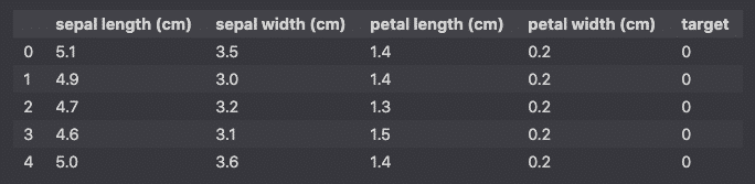
Load a dataset with Scikit-learn
Scikit-learn has a variety of built-in datasets that you can load like this:
import pandas as pd
from sklearn.datasets import load_iris

dataset = load_iris()
df = pd.DataFrame(dataset.data, columns=dataset.feature_names)
df['target'] = pd.Series(dataset.target)
df.head()
Sklearn Built-in datasets
Here are some of the methods that you can use to load more datasets.
load_boston()
load_breast_cancer()
load_diabetes()
load_iris()
load_wine()
Fetch openml
You can also use fetch_openml() to query open datasets.
from sklearn.datasets import fetch_openml
X, y = fetch_openml("titanic", version=1, as_frame=True, return_X_y=True)
X.head()
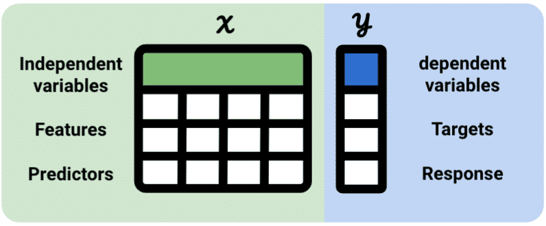
Data Representation in Sklearn
Data representation in scikit-learn is represented in X and y.
X= Independent variable = feature = predictor variabley= Dependent variable = target = response variable
In supervised learning, the scikit-learn tabular dataset has both independent and dependent (X and y) variables.
In unsupervised learning, the dependent (y) variable is unknown.
Data Formatting Requirements
When using the Scikit-learn api, the data should follow certain requirements:
- Data should be stored as numpy arrays or pandas dataframes
- The dependent variables
yshould be converted to continuous values (no categorical variables). - Missing values should be filled or removed
- Each
Xcolumn should be a unique independent variable - Each row should be an observation of the variable
- There should be as many labels as there are observations of a feature
Thus, preprocessing is critical when using Scikit-learn.
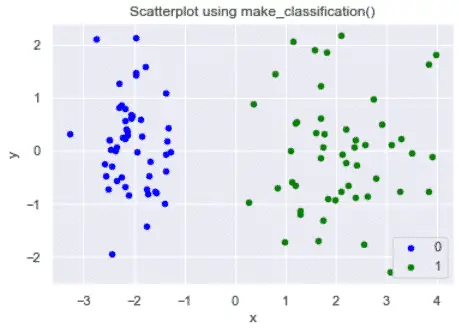
Generate Dummy Data
Libraries used: matplotlib, pandas, seaborn, sklearn
import matplotlib.pyplot as plt
import pandas as pd
import seaborn as sns

from sklearn.datasets import make_classification

sns.set()

# generate dataset for classification
X, y = make_classification(n_samples=100, n_classes=2, n_features=5, n_redundant=0, n_repeated=0, n_clusters_per_class=1,class_sep=2,random_state=42)

# prepare data for plot
df = pd.DataFrame(dict(x=X[:,0], y=X[:,1], label=y))
data = df.groupby('label')

# plot classification into a scatter plot
fig, ax = plt.subplots()
params = {0:'blue',1:'green'}
for key, value in data:
    value.plot(ax=ax,kind='scatter',x='x',y='y',label=key,color=params[key])

plt.title('Scatterplot using make_classification()')
plt.show()
Understand Scikit-learn machine learning models
The basic steps to run a machine learning model in Scikit-learn are:
- Load the dataset
- Define the machine learning model object*
- Define the feature variables and the target
- Split into training and testing data
- Use
.fit()to train the model. The process of training the data is also called “fitting”. - Use
.predict()to predict outcomes from the learned model - Evaluate the model
*Machine learning models in Scikit-learn are all created by Python classes (see: Object Oriented Programming).
A lot more steps can be added to make the model better, but we will focus on these as part of this tutorial.
Run your First Machine Learning Model in Scikit-learn
Now, lets train the most basic machine learning model with Scikit-learn and evaluate the performance using the classification report of sklearn.metrics.
import pandas as pd

from sklearn.datasets import load_breast_cancer
from sklearn.neighbors import KNeighborsClassifier
from sklearn.metrics import classification_report

# Load data
dataset = load_breast_cancer()
df = pd.DataFrame(dataset.data,columns=dataset.feature_names)
df['target'] = pd.Series(dataset.target)

# Define predictor and predicted datasets
X = df.drop('target', axis=1).values
y = df['target'].values

# Choose the machine learning model
knn = KNeighborsClassifier(n_neighbors=8)

# Train the model
knn.fit(X, y)

# Compute the prediction
y_pred = knn.predict(X)

# Print first 10 prediction labels
print(['Malignant' if x==0 else 'Benign' for x in y_pred[:10]])
Congratulations, you have run your first machine learning model in Scikit-learn.
This model, however, isn’t perfect.
Since we used the entire dataset to predict, it is hard to evaluate its quality on unseen data.
It would be best to split the dataset into training and testing data and evaluate the accuracy of the prediction on the test data.
Split the Data into testing and training data
To make sure our model is good when used on unseen data, it is good practice to split the dataset into training and testing datasets.
We will:
- split the data into training and testing sets
- train the model on the training set, leaving the testing set as is
- make a prediction using the test features
- compare the expected predictions with the real untouched test set
Using the code above, we will use the train_test_split method to create the training and testing splits.
On top of the X and y data, we add two parameters to train_test_split method: test_size and random_state.
The test_size parameter tells the percentage of data that we want to use for training as float.
The random_state parameter is used for replication. It says that the random numbers generated will remain in the same sequence so that another user can run your code and get the same results.
import pandas as pd
from sklearn.datasets import load_breast_cancer
from sklearn.neighbors import KNeighborsClassifier
from sklearn.metrics import classification_report
from sklearn.model_selection import train_test_split

# Load data
dataset = load_breast_cancer()
df = pd.DataFrame(dataset.data,columns=dataset.feature_names)
df['target'] = pd.Series(dataset.target)

# Define predictor and predicted datasets
X = df.drop('target', axis=1).values
y = df['target'].values

# Split into training and testing datasets
X_train, X_test, y_train, y_test = train_test_split(X, y, test_size=0.3, random_state=42)

# Choose the machine learning model
knn = KNeighborsClassifier(n_neighbors=8)
# Train the model
knn.fit(X_train, y_train)

# Compute the prediction
y_pred = knn.predict(X_test)

# compute accuracy of the model
knn.score(X_test, y_test)
This tells us that the accuracy of the model is
0.9649122807017544
Evaluate the Model
It is always important to evaluate the quality of the model.
To do so, we will plot the:
- Classification report
- Confusion Matrix
Classification Report
The classification report is a good way to compute the accuracy of your model.
from sklearn.metrics import classification_report

print(classification_report(y_test, y_pred))
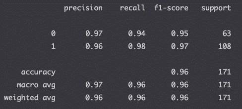
Read this article if you don’t know how to interpret the classification report.
Confusion Matrix
The confusion matrix computes the True positives, False positives, True negatives and False negatives of your machine-learned predictions.
import matplotlib.pyplot as plt
from sklearn.metrics import plot_confusion_matrix

color = 'white'
matrix = plot_confusion_matrix(knn, X_test, y_test, cmap=plt.cm.Blues)
matrix.ax_.set_title('Confusion Matrix', color=color)
plt.xlabel('Predicted Label', color=color)
plt.ylabel('True Label', color=color)
plt.gcf().axes[0].tick_params(colors=color)
plt.gcf().axes[1].tick_params(colors=color)
plt.show()
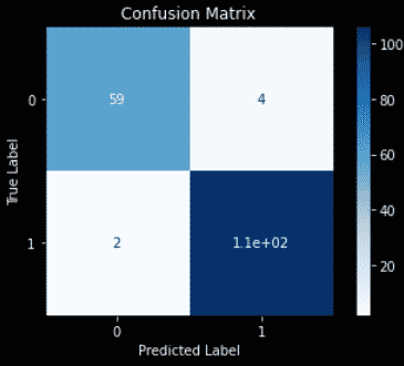
Read this article if you don’t know how to interpret the confusion matrix.
Advanced Scikit-learn
Machine learning models can be improved in many ways. This article was just an overview of Scikit-learn, so I have created a series of tutorials to help you improve your Machine learning skills.
- Generate dummy data with Scikit-learn
- Data preprocessing
- Train test split
- Pipeline
- Classification with Sklearn
- Regression in scikit-learn
- Evaluation of the model
Interesting Tutorials on Scikit-Learn
- Sklearn Tutorial Python (by Ander Fernández Jauregui)
Most common Scikit-Learn Libraries
- sklearn.datasets
- fetch_openml
- load_*
- make_classification
- sklearn.decomposition
- sklearn.model_selection
- train_test_split
- GridSearchCV
- cross_val_score
- sklearn.neighbors
- sklearn.linear_model
- LinearRegression
- LogisticRegression
- Ridge
- Lasso
- ElasticNet
- sklearn.tree
- sklearn.ensemble
- VotingClassifier
- RandomForestClassifier
- RandomForestRegressor
- BaggingClassifier
- BaggingReggressor
- AdaBoostClassifier
- AdaBoostRegressor
- GradientBoostingClassifier
- GradientBoostingRegressor
- StackingClassifier
- sklearn.svm
- LinearSVC
- SVC
- SVR
- sklearn.naive_bayes
- GaussianNB
- sklearn.cluster
- sklearn.impute
- SimpleImputer
- sklearn.feature_extraction
- CountVectorizer
- TfidfTransformer
- TfidfVectorizer
- sklearn.preprocessing
- OneHotEncoder
- MinMaxScaler
- StandardScaler
- sklearn.metrics
- mean_squared_error
- accuracy_score
- roc_auc_score
- classification_report
- plot_confusion_matrix
- plot_roc_curve
- sklern.pipeline
- make_pipeline
- Pipeline
Conclusion
This is the end of the introduction to Scikit-learn. We have seen what Scikit-learn is and how to use it in your machine learning projects.

SEO Strategist at Tripadvisor, ex- Seek (Melbourne, Australia). Specialized in technical SEO. Writer in Python, Information Retrieval, SEO and machine learning. Guest author at SearchEngineJournal, SearchEngineLand and OnCrawl.