Decision trees are predictive machine learning models that use simple binary rules to predict the value of a target variable.
Navigation
Show
What is a Decision Tree?
A Decision tree is a data structure consisting of a hierarchy of nodes that can be used for supervised learning and unsupervised learning problems (classification, regression, clustering, …).
Decision trees use various algorithms to split a dataset into homogeneous (or pure) sub-nodes.
Advantages of decision trees
Decision tree algorithms have multiple advantages:
- Simple to understand and interpret
- Flexible as they can describe non-linear data
- Simple to use as no data preprocessing needed.
On the other hand, trees do have some disadvantages:
- Sensitive to small variations in the training data
- Susceptible to overfitting when unconstrained
Understand the Decision Tree Algorithm
Decision trees are simple models that have branches, nodes and leaves and break down a dataset into smaller subsets containing instances with similar values.
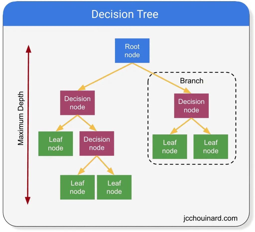
Decision Trees Definitions
- Root node: First node in the path from which all decisions initially started from. It has no parent node and 2 children nodes
- Decision nodes: Nodes that have 1 parent node and split into children nodes (decision or leaf nodes)
- Leaf nodes: Nodes that have 1 parent, but do not split further (also known as terminal nodes). They are the nodes that produce the prediction.
- Branches: A subsection of the entire tree (also known as a sub-tree)
- Parent / child nodes: A node that is divided in sub-nodes is called a parent node. The sub-nodes are the child nodes of the parent from which they divided.
- Maximum depth: maximum number of branches between the top and the lower end
Types of Decision Tree Algorithms
There are multiple decision tree algorithms:
- ID3 (Iterative Dichotomiser 3)
- C4.5 (extension of ID3)
- CART (Classification And Regression Tree)
- Chi-square (Chi-square automatic interaction detection)
- MARS (Multivariate Adaptive Regression Splines)
There are 2 decision trees grouped under Classification and decision tree (CART).
- Classification decision tree (used for categorical data)
- Regression decision tree (used for continuous data)
Some techniques use more than one decision tree. They are called ensemble learning algorithms.
Decision Tree Metrics
Decision trees try to produce the purest leaves in a recursive way by splitting nodes into smaller sub-nodes.
But how does it choose how to split the nodes, evaluate the purity of a leaf, or decide when to stop?
- Measure the quality of a split: gini or entropy
- Identify with feature and which split point: Information Gain (IG), Reduction in variance
For decision tree classification problems on categorical variables:
- Entropy and Information Gain (IG)
- Gini impurity
For decision tree regression problems on continuous variables:
- Reduction in variance
Information Gain (IG)
To produce the “best” result, decision trees aim at maximizing the Information Gain (IG) after each split.
Information Gain of a single node is calculated by subtracting the entropy to 1.

The information gain helps define if the split contains more pure nodes compared to the parent node.
To measure the information gain of a parent against its children, we must subtract the weighted entropy of the children from the entropy of the parent.

But, what is entropy?
Entropy
Entropy is used to measure the quality of a split for categorical targets.
The formula of entropy in decision trees is:

Where pi represents the percentage of the class in the node.
Below is a representation of the calculation of the entropy on a dataset where there are 2 values in the class split in 30%-70%.
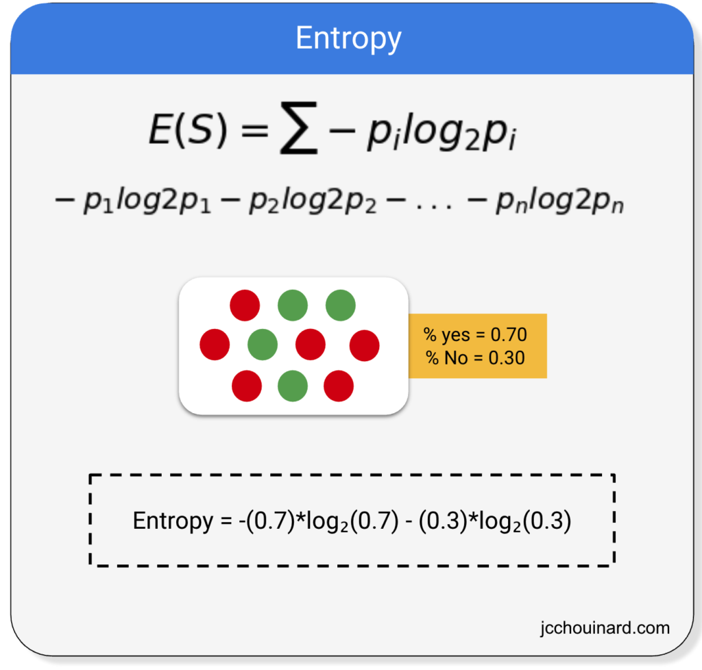
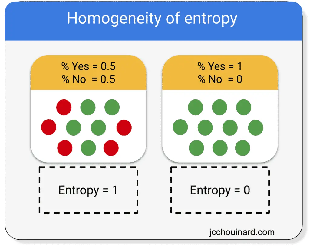
The smaller the entropy, the higher the homogeneity of the nodes.
To calculate the entropy of a split, we:
- Calculate the entropy of the parent node
- Calculate the entropy of the children nodes
- Calcute the weighted average entropy of the split
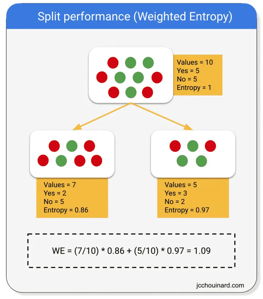
If the weighted entropy is smaller than the entropy of the parent node, then the information gain is greater.
Above, the entropy of the parent equals 1 and the weighted entropy equals 1.09.
So, in the formula:
The information gain is equal to:
IG = 1 - 1.09 = -0.09
Interpretation of the information gain
A split like the one above would reduce the entropy.
The decision tree tries to maximize the information gain.
Therefore, the split would not be made.
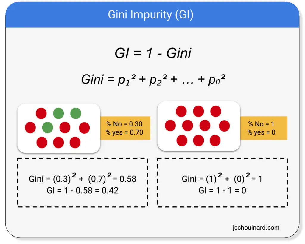
Gini Impurity
Gini impurity is used as an alternative to information gain (IG) to compute the homogeneity of a leaf in a less computationally intensive way.
The purer, or homogenous, a node is, the smaller the Gini impurity is.
The way Gini impurity works is by:
- Selecting elements at random and atributing the same class
- Computing the probability of incorrecty classifying a randomly chosen element
Gini is the sum of squares of probabilities for each class.
And, then, again, the model will estimate the purity of the split by computing the weighted Gini impurity of both children leaves compared to the Gini impurity of the parent.

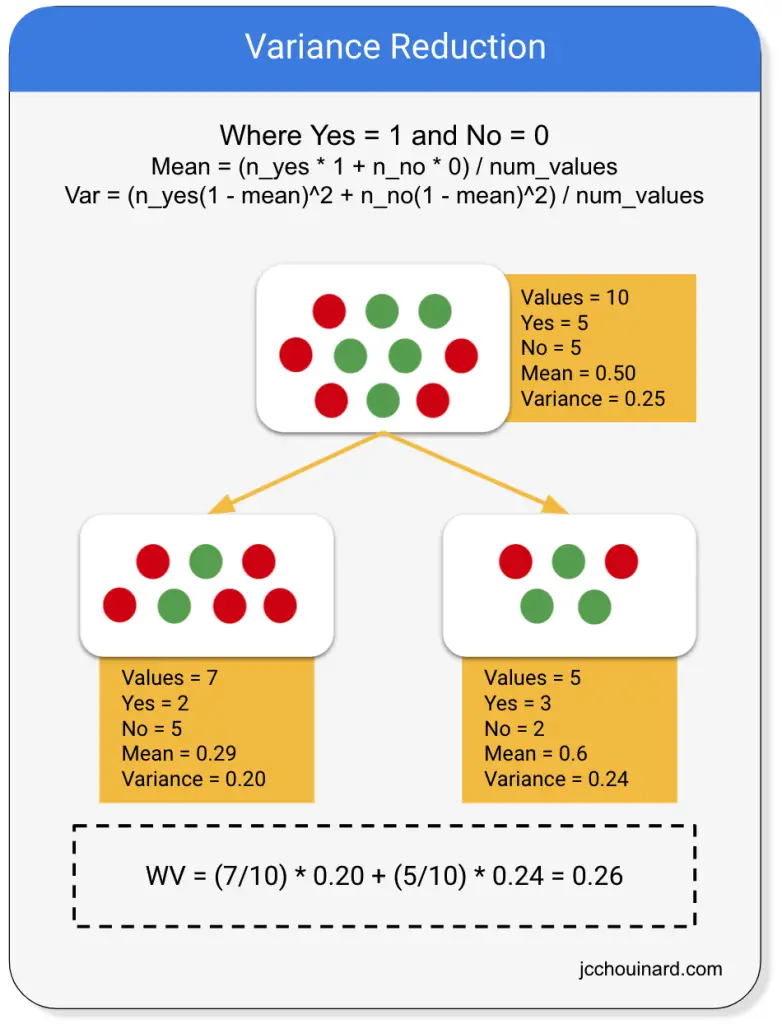
Variance Reduction
Variance reduction, or mean square error, is a technique used to estimate the purity of the leaves in a decision tree when dealing with continuous variables.
While decision trees can estimate the homogeneity of leaves using the entropy / information gain or Gini impurity on categorical variables they calculate the reduction in variance to estimate the purity of leaves on continuous variables.
Decision Tree Classification in Scikit-Learn
The decision tree classification has the objective of inferring the class labels.
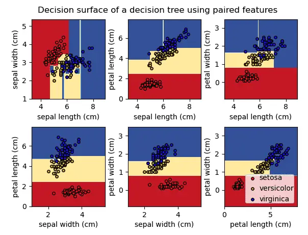
As you can see in the graph above, the decision tree returns an orthogonal decision boundary (not curved) and help predict labels on a non-linear dataset.
The decision tree classification will define decision regions based on the somewhat rectangular decision boundaries.
Use DecisionTreeClassifier to make a decision tree classification in Scikit-learn.
Below:
max_depth: limits the model to X levels of depths, even if maximum purity isn’t reachedcriterion: let’s you define the way to estimate the purity of the leaf (e.g.giniorentropy)
import numpy as np

from sklearn.datasets import make_classification
from sklearn.metrics import accuracy_score
from sklearn.model_selection import train_test_split
from sklearn.tree import DecisionTreeClassifier

# Define random state for reproducible results
np.random.seed(1)

# Generate dummy dataset
X, y = make_classification(
    n_samples=200,
    n_features=4,
    n_classes=2)

# Split into training and test sets
X_train, X_test, y_train, y_test = train_test_split(
                                                X,
                                                y,
                                                stratify=y)

# Instantiate a decision tree classifier
# And choose a 'critierion' to estimate
# the impurity of a node
dt = DecisionTreeClassifier(
    max_depth=3,
    criterion='gini'
    )

# Train the classifier
dt.fit(X_train, y_train)

# Predict the labels of the test set
y_pred = dt.predict(X_test)

# Evaluate the accuracy score
accuracy_score(y_test, y_pred)
Decision Tree Regression
The decision tree regression is based on the decision tree algorithm.
The decision tree regression will fit a sine curve to the data to define the rules of the classification or the regression.
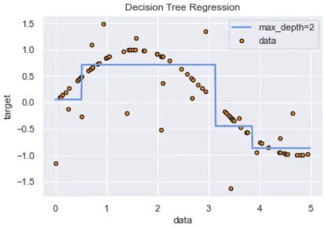
However, decision trees can overfit the model by interpreting too granular details from training data depending on the chosen hyperparameters.
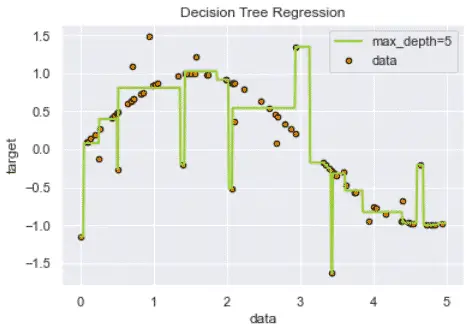
This overfitting can be minimized using ensemble methods instead (e.g. random forest).
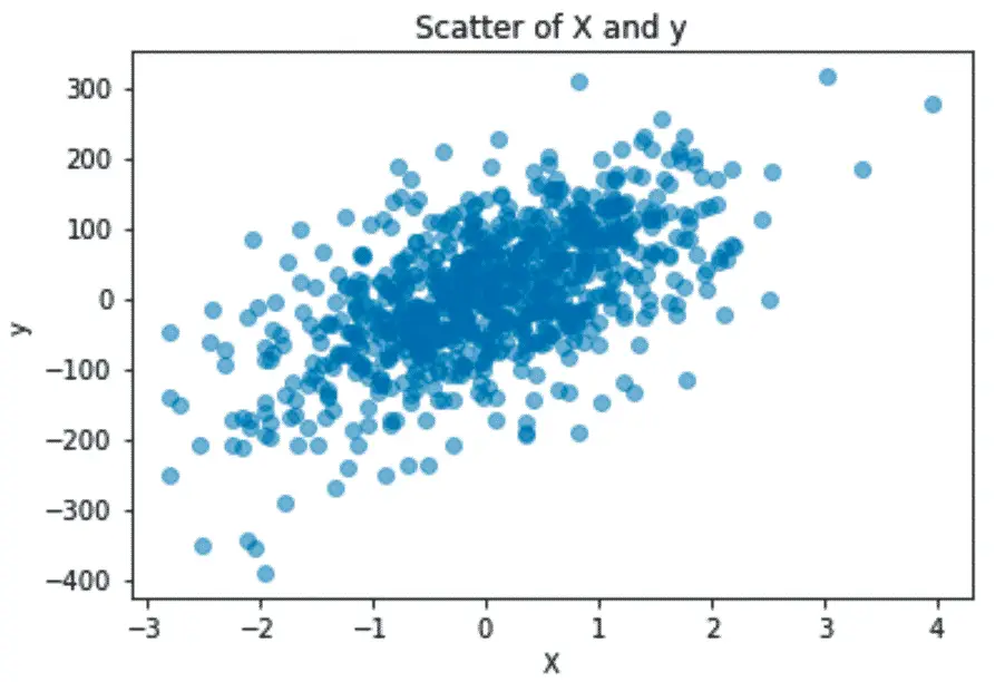
Use DecisionTreeRegressor to make a decision tree regression in Scikit-learn.
First, create and visualize the regression data.
import numpy as np
import matplotlib.pyplot as plt

from sklearn.datasets import make_regression

# Define random state for reproducible results
np.random.seed(1)

# Generate dummy dataset
X, y = make_regression(
    n_samples=200,
    n_features=4,
    n_targets=4,
    bias=2,
    noise=20)

# Plot the data
plt.scatter(X, y, alpha=0.5)
plt.xlabel('X')
plt.ylabel('y')
plt.title('Scatter of X and y')
plt.show()
Next, split into test and training sets and run the DecisionTreeRegressor algorithm.
from sklearn.model_selection import train_test_split
from sklearn.tree import DecisionTreeRegressor

# Split into training and test sets
X_train, X_test, y_train, y_test = train_test_split(
                                    X,
                                    y,
                                    test_size=0.3
                                    )


# Instantiate a decision tree regressor
dt = DecisionTreeRegressor(
    max_depth=5
    )

# Train the classifier
dt.fit(X_train, y_train)

# Predict the labels of the test set
y_pred = dt.predict(X_test)
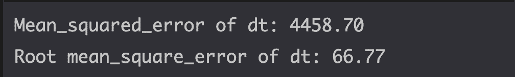
Finally, estimate the model performance using the mean_squared_error.
from sklearn.metrics import mean_squared_error as MSE
# Compute mean squared error
mse_dt = MSE(y_test, y_pred)

# Compute Root Mean Squared Error (RMSE)
rmse_dt = mse_dt ** (1/2)

# Results
print(f'Mean_squared_error of dt: {mse_dt:.2f}')
print(f'Root mean_square_error of dt: {rmse_dt:.2f}')
Alternatives to Decision Trees
Decision trees can often overfit the data.
A great alternative to decision trees is ensemble learning, with algorithms such as:
- Random Forests
- Gradient Boosting Machines (GBM)
- Bootstrap Aggregation
- Adaboost
Interesting Work from the Community
- Visualize a Decision Tree in 4 Ways with Scikit-Learn and Python (by Piotr Płoński)
- A pragmatic dive into Random Forests and Decision Trees with Python
- Generating Synthetic Classification Data using Scikit
- 4 Simple Ways to Split a Decision Tree in Machine Learning
Conclusion
Bravo, you made it this far.
We have covered quite a lot.
We have learned:
- the basics of decision trees
- the different decision tree algorithms that can be used for classification and regression problems.
- how each model estimates the purity of the leaf.
- how each model can be biased and lead to overfitting of the data
- how to run decision tree machine learning models using Python and Scikit-learn.
Next, we will cover ensemble learning algorithms.

SEO Strategist at Tripadvisor, ex- Seek (Melbourne, Australia). Specialized in technical SEO. Writer in Python, Information Retrieval, SEO and machine learning. Guest author at SearchEngineJournal, SearchEngineLand and OnCrawl.