Preprocessing Data With SCIKIT-LEARN (Python tutorial)

Data preprocessing is an important step in the machine learning workflow. The quality of the data makes the difference between a good model and a bad model.

In this tutorial, we will learn how to do data preprocessing with Scikit-learn executing a logistic regression on the Titanic dataset

What is Data Preprocessing?

Data preprocessing is the process of transforming data into a useful, manageable and understandable format.

Why Data Preprocessing?

Preprocessing is important to remove noise in the data and make sure that it is in a usable format for your machine learning library. What is handled in data preprocessing:

• Missing data: Remove, fix and impute missing data
• Feature engineering: Infer additional features from raw data
• Data formatting: The data might not be in the format that you need. For example, the Scikit-learn API requires the data to be a Numpy array or a pandas DataFrame.
• Scaling the data: The data may not all be on the same scale. For instance, kilograms and pounds can be put on same scale from 0 to 1.
• Decomposition: i.e. keep only hour of the day from datetime
• Aggregation: i.e. aggregate by loggedin vs non logged in

Requirements of the Scikit-learn API

The sklearn api has some requirements on what kind of data it will process.

• data stored as numpy arrays or pandas dataframes
• continuous values (no categorical variables)
• no missing values
• each column should be a unique predictor variable (or feature)
• each row should be an observation of the feature
• there should be as many labels as there are observations of a feature

Data Preprocessing in Scikit-learn

In this tutorial, we will use the Titanic dataset to execute data preprocessing in an integrated project with Scikit-learn.

Preprocessing steps:

1. Load data with Scikit-learn
2. Exploratory data analysis
3. Handle missing values
4. Infer new features with feature engineering
5. Encode categorical features
6. Scale numeric features
7. Create a LogisticRegression
8. Build a pipeline

1. Load the data

We will use the Titanic dataset as this is a common dataset used when learning data science.

You can load the titanic dataset using fetch_openml().

import pandas as pd
from sklearn.datasets import fetch_openml

df = fetch_openml('titanic', version=1, as_frame=True)['data']
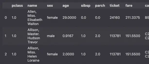
df.head(3)

2. Perform Exploratory Data Analysis

Data preprocessing is generally the step that comes after exploratory data analysis in the data science process. The techniques of EDA can be used to make unexpected discoveries on the data that may require data preprocessing.

We will conduct exploratory data analysis to identify null columns, find missing values and handle various data types.

Validate Numeric Values

The info() method can be used to show potentially wrong data types in a Pandas DataFrame.

df.info()

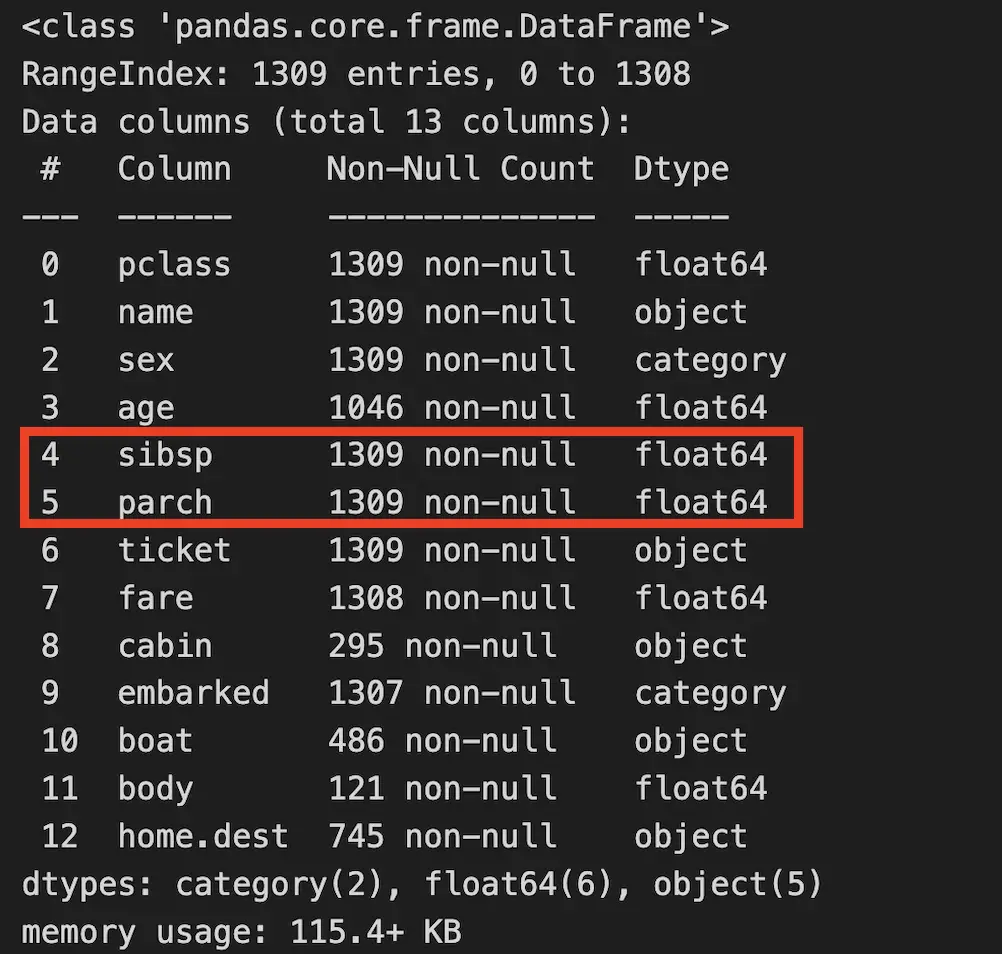
For instance, data preprocessing may be used here to convert floating numbers to integers. Why would we keep floating numbers on parents and siblings while it is not possible to have 0.5 parent.

# Validate Numberic Data
df['sibsp'] = df['sibsp'].astype(int)  # siblings
df['parch'] = df['parch'].astype(int)  # parents/children

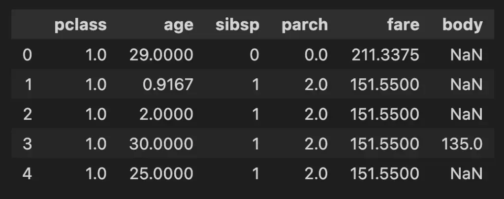
We can also select a subset of the columns that are numeric:

# Validate Dtypes
df.select_dtypes('number').head()

Validate Categorical Data

We can use exploratory data analysis techniques to identify if we need data preprocessing on the categorical data.

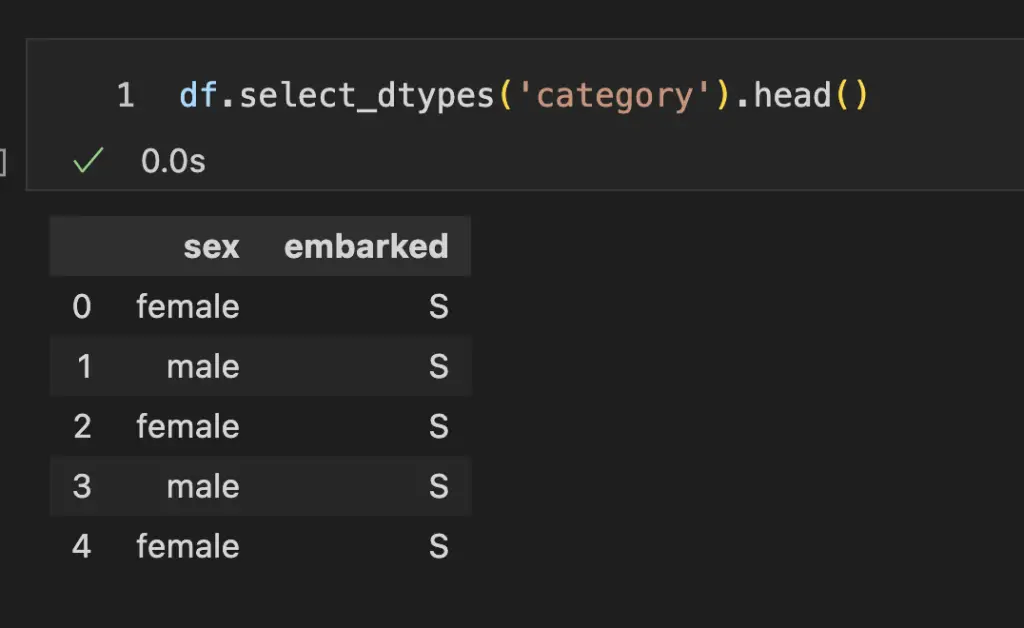
Show categorical columns with select_dtypes:

# Validate Dtypes
df.select_dtypes('category').head()

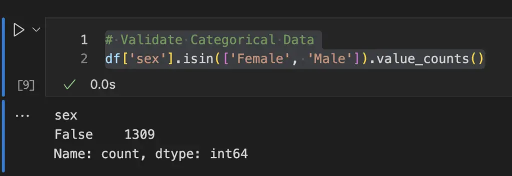
We can validate the categorical data using the isin() and the value_counts() methods on the categorical column of the pandas dataframe.

# Validate Categorical Data
df['sex'].isin(['Female', 'Male']).value_counts()

Show null columns

The info() method can be used to show null value count by column in Pandas.

df.info()

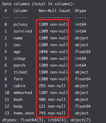
All columns have value in them.

Show missing values

df.isnull().sum()

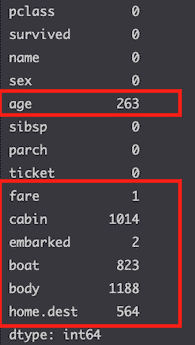
A lot of columns are missing values. But how important is that actually?

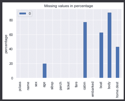
Let’s pot and apply seaborn style.

import seaborn as sns
sns.set()
miss_vals = pd.DataFrame(df.isnull().sum() / len(df) * 100)
miss_vals.plot(kind='bar',title='Missing values in percentage',ylabel='percentage')

3. Handle Missing Data

We can handle missing data in two ways:

• Remove it (dropping)
• Imputing it from the whole dataset (using the mean, median, mode…)

Dropping missing data

You could drop rows and columns with missing values, at risk of losing too much information.

print(f'Size of the dataset: {df.shape}')
df.drop(['cabin', 'boat', 'body', 'home.dest'], axis=1, inplace=True)
df.dropna(inplace=True)
print(f'Size of the dataset after dropping: {df.shape}')

However, it is preferable to impute data from the entire dataset.

Imputing missing data

Imputing missing data relates to using subject-matter expertise to replace missing data with educated guesses.

You can replace missing values of categorical variables by using the most common value (mode), or the mean for numerical variables.

Just note that it is important to split the dataset into training and testing set before imputing values in order to avoid data leakage.

Both pandas and sklearn can be used to fill missing values. Here we have:

import pandas as pd
from sklearn.datasets import fetch_openml

df = fetch_openml('titanic', version=1, as_frame=True)['data']
print(f'Number of null values in the age column: {df.age.isnull().sum()}')

Here we have 263 null values to handle in the age column.

Imputing with Pandas

Fill in missing data using the fillna() method with the mean of the column as the parameter.

import pandas as pd
from sklearn.datasets import fetch_openml

df = fetch_openml('titanic', version=1, as_frame=True)['data']

df['age'].fillna(df['age'].mean(), inplace=True)
print(f'Number of null values: {df.age.isnull().sum()}')

Imputing with Scikit-learn

Scikit-learn imputers, also known as transformers, can be used to fill missing values.

Using SimpleImputer we will replicate the operation we did in pandas to fill missing values with the mean of the age column.

Simple transformation

The SimpleImputer class works with the fit_transform method that executes both the fit() and the transform() methods in a single line.

from sklearn.datasets import fetch_openml
from sklearn.impute import SimpleImputer

df = fetch_openml('titanic', version=1, as_frame=True)['data']

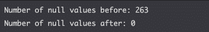
print(f'Number of null values before: {df.age.isnull().sum()}')

imp = SimpleImputer(strategy='mean')
df['age'] = imp.fit_transform(df[['age']])

print(f'Number of null values after: {df.age.isnull().sum()}')

The missing_values keyword

Sometimes, the missing values are not in the nan format.

print('Data types of missing values')
for col in df.columns[df.isnull().any()]:
    print(col, df[col][df[col].isnull()].values[0])

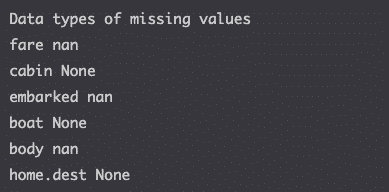
You can deal with different types of missing values using the missing_values keyword.

from sklearn.datasets import fetch_openml
from sklearn.impute import SimpleImputer

df = fetch_openml('titanic', version=1, as_frame=True)['data']

imp = SimpleImputer(missing_values=None,strategy='most_frequent')
df['cabin'] = imp.fit_transform(df[['cabin']])

df.cabin.isnull().sum()

Fill in missing values of the whole dataset

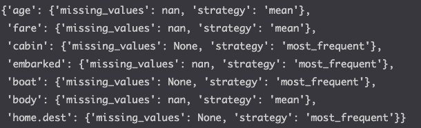
Create a function to define the parameters to be used in the SimpleImputer() class.

def get_parameters(df):
    parameters = {}
    for col in df.columns[df.isnull().any()]:

        if df[col].dtype == 'float64' or df[col].dtype == 'int64' or df[col].dtype =='int32':
            strategy = 'mean'
        else:
            strategy = 'most_frequent'
        missing_values = df[col][df[col].isnull()].values[0]
        parameters[col] = {'missing_values':missing_values, 'strategy':strategy}
    return parameters
get_parameters(df)

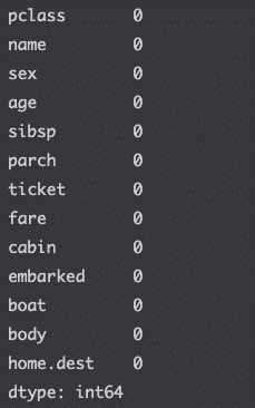
Then, loop through each column to transform it.

from sklearn.datasets import fetch_openml
from sklearn.impute import SimpleImputer

df = fetch_openml('titanic', version=1, as_frame=True)['data']

parameters = get_parameters(df)

for col, param in parameters.items():
    missing_values = param['missing_values']
    strategy = param['strategy']
    imp = SimpleImputer(missing_values=missing_values,strategy=strategy)
    df[col] = imp.fit_transform(df[[col]])

df.isnull().sum()

Different kinds of missing values

Sometimes missing values will be encoded differently. For example, missing values could have been filled using a question mark ?. These cases require additional data manipulation. Here are some examples.

import numpy as np
import pandas as pd

df[df == 9999] = np.nan  # values too large to be true
df[df.str.contains('error')] = np.nan # error messages added by computer programs
df[df == '?'] = np.nan # human decisions on how they wanted to handle missing data

4. Create New Features (Feature Engineering)

Feature engineering is the process of using domain knowledge to extract features from raw data.

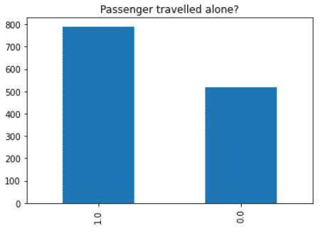
For example, we can use feature engineering to infer if the person travelled alone by looking at who they travelled with.

• SibSp captures the number of siblings that the passengers travelled with.
• Parch captures the number of parents and children that the passengers travelled with.

By combining each, we can find out if they travelled alone.

from sklearn.datasets import fetch_openml

df = fetch_openml('titanic', version=1, as_frame=True)['data']

df['family'] = df['sibsp'] + df['parch']
df.loc[df['family'] > 0, 'travelled_alone'] = 0
df.loc[df['family'] == 0, 'travelled_alone'] = 1
df['travelled_alone'].value_counts().plot(title='Passenger travelled alone?',kind='bar')

5. Encode Categorical Geatures

When dealing with classification problems, you need to encode categorical features numerically on a continuous scale.

The Scikit-learn API requires categorical features to be converted into binary arrays (0s, 1s).

There are two ways that we can achieve this.

• sciki-learn: OneHotEncoder()
• pandas: get_dummies()

Encoding categorical features with Scikit-learn

To convert categorical features with Scikit-learn, use OneHotEncoder() with the fit_transform() method.

import pandas as pd 

from sklearn.datasets import fetch_openml
from sklearn.preprocessing import OneHotEncoder

df = fetch_openml('titanic', version=1, as_frame=True)['data']

df[['female','male']] = OneHotEncoder().fit_transform(df[['sex']]).toarray()
df[['sex','female','male']] 

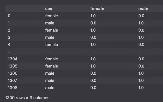
But this is redundant. All this information could be stored in a single column where female is 0 and male is 1 (or vice versa).

To do so, well select the Male column from the array resulting from the fit_transform method.

import pandas as pd 

from sklearn.datasets import fetch_openml
from sklearn.preprocessing import OneHotEncoder

df = fetch_openml('titanic', version=1, as_frame=True)['data']
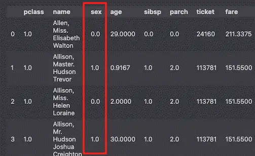
df['sex'] = OneHotEncoder().fit_transform(df[['sex']]).toarray()[:,1]
df.head() 

Now we only have one usable sex column, encoded in binaries where 0 == female and 1 == male.

Encoding categorical features with Pandas

The alternative to OneHotEncoder is the pandas get_dummies() method.

To replicate the same thing we just did is much simpler in pandas, by selecting the column to encode and using the drop_first keyword to remove redundant features.

import pandas as pd 

from sklearn.datasets import fetch_openml

df = fetch_openml('titanic', version=1, as_frame=True)['data']

df['sex'] = pd.get_dummies(df['sex'],drop_first=True)

df.head(3)

Encoding all categorical features

Since this is a tutorial on Scikit-learn, I will use OneHotEncoder to convert all categorical features to binary format.

What we will do is:

1. Load data
2. Select categorical columns using the select_dtypes(include=['category']) method
3. Create a loop to iterate through each of the selected columns. For each column:
   • Impute missing values
   • Create a list of the feature’s labels
   • Use this list as column headers where to add the resulting array from OneHotEncoder
   • Drop the redundant columns

import pandas as pd 

from sklearn.datasets import fetch_openml
from sklearn.preprocessing import OneHotEncoder

df = fetch_openml('titanic', version=1, as_frame=True)['data']

# Select columns which dtype == 'category'
cat_cols = df.select_dtypes(include=['category']).columns
print(f'Categorical columns: {cat_cols}')

# Loop through each categorical column 
for col in cat_cols:
    # Impute missing values
    fill_value = df[col].mode()[0] 
    df[col].fillna(fill_value, inplace=True)
    
    # create a list of labels to be encoded in the column
    append_to = list(df[col].unique())

    # These labels will be use as column headers
    print(append_to)

    # Apply OneHotEncoder()
    df[append_to] = OneHotEncoder().fit_transform(df[[col]]).toarray()

    # Drop non-encoded column
    df.drop(col, axis=1, inplace=True)

    # Drop redundant data
    df.drop(append_to[0], axis=1, inplace=True)

print(df.columns)
df[['male','C','Q']].head(3)

We now see new columns where the male column shows the encode sex feature and the C and Q the encoded embarked feature.

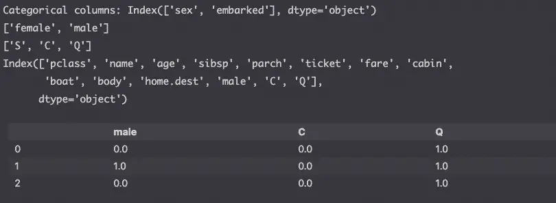
There were 3 different port of embarkation (C = Cherbourg; Q = Queenstown; S = Southampton) in the Titanic dataset, but now we have two columns (C and Q).

Why?

Because, we can infer that when the port of embarkation isn’t Q or S, it is C. Thus, we removed the first feature as it was redundant.

6. Scale Numeric Features

In different datasets, the ranges within features are not necessarily the same.

For example, one feature can should data in pounds and the other in kilograms.

To interpret properly, these features need to be on the same scale

So, we need to normalize the data.

To normalize the data, we can use MinMaxScaler or StandardScaler:

• MinMaxScaler transforms each feature to a given range (e.g. from 0 to 1)
• StandardScaler standardizes the features by removing the mean and scaling to unit variance so that each feature has μ = 0 and σ = 1.

We are going to do a series of steps to applly both classes:

1. Load data
2. Select numeric columns using the select_dtypes(include=['int64', 'float64', 'int32']) method
3. Create a loop to impute missing values on each numeric column. For each column:
4. Apply the scaler class

MinMaxScaler

MinMaxScaler() put all numeric values on a scale from 0 to 1.

Let’s apply the model and see how it impacts the data.

from sklearn.datasets import fetch_openml
from sklearn.preprocessing import MinMaxScaler

df = fetch_openml('titanic', version=1, as_frame=True)['data']

# Select numerical columns
num_cols = df.select_dtypes(include=['int64', 'float64', 'int32']).columns
print(num_cols)

# Impute missing values
for col in num_cols:
    fill_value = df[col].mean()
    df[col].fillna(fill_value, inplace=True)

# Apply MinMaxScaler
minmax = MinMaxScaler()
df[num_cols] = minmax.fit_transform(df[num_cols])
df[num_cols]

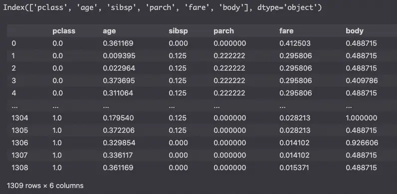
Above, we can see that all the values are scaled from 0 to 1.

StandardScaler

StandardScaler()put all numeric values on a scale where the mean equals 0 and the standard deviation equals 1.

Let’s apply the model and see how it impacts the data.

from sklearn.datasets import fetch_openml
from sklearn.preprocessing import StandardScaler

df = fetch_openml('titanic', version=1, as_frame=True)['data']

# Select numerical columns
num_cols = df.select_dtypes(include=['int64', 'float64', 'int32']).columns
print(num_cols)

# Impute missing values
for col in num_cols:
    fill_value = df[col].mean()
    df[col].fillna(fill_value, inplace=True)

# Apply StandardScaler
ss = StandardScaler()
df[num_cols] = ss.fit_transform(df[num_cols])
df[num_cols].describe()

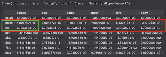
Using the describe() method, we can look at the mean and standard deviation of the scaled numeric columns.

The mean does not look to equal 0 but in fact, 4.995749e-15 equals 0.000000000000004995749. This is so close to 0 that it can be considered to be equal 0. The same goes with the standard deviation that is so close to 1 that it can be considered equal to 1.

7. Create a LogisticRegression

Now, let’s create a logistic regression from the dataset. For the purpose of simplicity, I will not add training and testing datasets. I just want to show how to run a basic logistic regression machine learning model with Scikit-learn.

from sklearn.datasets import fetch_openml
from sklearn.linear_model import LogisticRegression

X, y = fetch_openml('titanic', version=1, as_frame=True, return_X_y=True)

# impute missing values
X['age'].fillna(X['age'].mean(), inplace=True)
X['embarked'].fillna(X['embarked'].mode(), inplace=True)

# handle categorical data
X = pd.get_dummies(X[['age','embarked', 'sex','pclass']],drop_first=True)

# fit machine learning model
model = LogisticRegression()
model.fit(X, y)

# make prediction
model.predict(X)

8. Building a Pipeline

Now, we have covered a lot. There is one last thing that I want to discuss is how to integrate all these steps into a Scikit-learn pipeline.

Building a pipeline would require a post of its own and we have already covered quite a lot.

Let’s just explain briefly what the code does and keep the details out.

Using the Pipeline class, we create a series of steps that we want to execute in order.

1. Load the dataset
2. Create a transformer to impute, then scale numeric data
3. Create a transformer to convert categorical data to binary
4. Define which transformer to apply to which column (numeric and categorical data need different preprocessing). Store as a preprocessor.
5. Add the preprocessor and the LogisticRegression() machine learning model to the steps of the Pipeline, in the order to be executed.
6. Create a training and testing datasets to be able to evaluate the model later.
7. Train the model using the fit() method.
8. Evaluate the model using the score() method.

from sklearn.datasets import fetch_openml
from sklearn.compose import ColumnTransformer
from sklearn.impute import SimpleImputer
from sklearn.linear_model import LogisticRegression
from sklearn.model_selection import train_test_split
from sklearn.pipeline import Pipeline
from sklearn.preprocessing import OneHotEncoder, StandardScaler

# load dataset
X, y = fetch_openml('titanic', version=1, as_frame=True, return_X_y=True)

# Impute and scale numeric data
numeric_features = ['age']
numeric_transformer = Pipeline(steps=[
    ('imputer', SimpleImputer(strategy='mean')),
    ('scaler', StandardScaler())])

# Convert categorical data to binary
categorical_features = ['embarked', 'sex', 'pclass']
categorical_transformer = OneHotEncoder(handle_unknown='ignore')

# Define which transformer to apply to which data
preprocessor = ColumnTransformer(
    transformers=[
        ('num', numeric_transformer, numeric_features),
        ('cat', categorical_transformer, categorical_features)])

# Add the transformers to the steps and execute the machine learning model
model = Pipeline(steps=[('preprocessor', preprocessor),
                      ('classifier', LogisticRegression())])

# Split into testing and training datasets
X_train, X_test, y_train, y_test = train_test_split(X, y, test_size=0.3,
                                                    random_state=42)

# Train the model on the training dataset
model.fit(X_train, y_train)

# evaluate the model by comparing results to the test dataset.
print(f'Model score: {model.score(X_test, y_test)}')

Conclusion

If you made it this far, you deserve big congratulations.

You have now completed this tutorial on data preprocessing with Scikit-learn.

Jean-Christophe Chouinard

SEO Strategist at Tripadvisor, ex- Seek (Melbourne, Australia). Specialized in technical SEO. Writer in Python, Information Retrieval, SEO and machine learning. Guest author at SearchEngineJournal, SearchEngineLand and OnCrawl.