k-Nearest Neighbors is a machine learning algorithm used in supervised learning to predict the label of data points by looking what is the majority in its closest neighbours.
This is a classification approach.
Given a number of neighbors k, the k-Nearest neighbors algorithm will look at what is present in the majority and will attribute the majority to the new data points.
Learn k-Nearest Neighbors
This post is an overview of the k-Nearest Neighbors algorithm and is in no way complete.
If you want to learn more about the k-Nearest Neighbors algorithms, here are a few Datacamp tutorials that helped me.
Understand the k-Nearest Neighbors algorithm visually
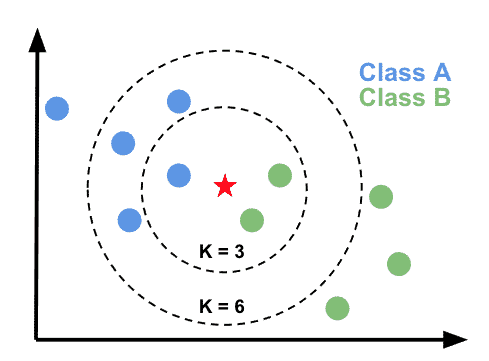
This visualization help understand how k-Nearest Neighbors work. Given a k value, what will be the prediction?
- In the
k=3circle,greenis the majority, new data points will be predicted asgreen; - In the
k=6circle,blueis the majority, new data points will be predicted asblue;
Advantages and Disadvantages of the KNN approach
Advantages: The k-Nearest Neighbors algorithm is simple to implement and robust to noisy training data.
Disadvantages: High cost of computation compared to other algorithms. Storage of data: memory based, so less efficient. Need to define which k value to use.
When to use the KNN algorithm?
- Image and video recognition
- Filtering of recommender systems
Run the k-Nearest Neighbors with Scikit-learn
Let’s run the k-Nearest Neighbors algorithm with Scikit-learn.
- Load data
- Split data into training and test sets
- Train the classifier model on the training set and make predictions on the test set
- Evaluate the model looking at the known labels.
- Fine-tune the model
Load data
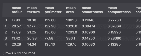
Sklearn has a set of built-in datasets that we can use. Here we will load the breast cancer dataset.
import pandas as pd
from sklearn import datasets

dataset = datasets.load_breast_cancer()
df = pd.DataFrame(dataset.data,columns=dataset.feature_names)
df['target'] = pd.Series(dataset.target)
df.head()
Let’s look at the labels that we will try to predict.
Based on all the features that we have:
print(dataset.feature_names)
# [
#     'mean radius',
#     'mean texture',
#     'mean perimeter',
#     ...,
#     'worst fractal dimension'
# ]
we will try to predict the severity of the breast cancer.
print(dataset.target_names)
# ['malignant', 'benign']
Split Data into Training and Test sets
Whenever we build a machine learning model, we want to check its accuracy.
You will need to split your data into training and test datasets using the train_test_split module.
- The training dataset is used to fit (or train) the model.
- The test dataset is excluded from training. It is labelled data that will be used to compare against the predictions made by the model.
from sklearn.model_selection import train_test_split

# Define independent (features) and dependent (targets) variables
X = dataset['data']
y = dataset['target']

# split taining and test set
X_train, X_test, y_train, y_test = train_test_split(X, y, test_size=0.3, random_state=42, stratify=y)
Train the Model and make predictions
Now, to make predictions based on the labelled data, we will:
- Initiate the
KNeighborsClassifierthe machine learning model - Use the
.fit()method to train the mode - Use the
.predict()method to make predictions
from sklearn.neighbors import KNeighborsClassifier

# train the model
knn = KNeighborsClassifier(n_neighbors=8)
knn.fit(X_train, y_train)
y_pred = knn.predict(X_test)
Evaluate the model
It is very important to evaluate the accuracy of the model. We can do this using the .score() method on the knn object.
# compute accuracy of the model
knn.score(X_test, y_test)
The accuracy of the model is
0.9239766081871345
Which is a pretty good result in this case.
Test Different K Values
We can also try to look at the model accuracy of multiple k values.
import numpy as np
import matplotlib.pyplot as plt

neighbors = np.arange(1, 25)
accuracy = np.empty(len(neighbors))

for i, k in enumerate(neighbors):
    knn = KNeighborsClassifier(n_neighbors=k)
    knn.fit(X_train, y_train)
    accuracy[i] = knn.score(X_test, y_test)

plt.title('k-NN accuracy by number of Neighbors')
plt.plot(neighbors, accuracy)
plt.xlabel('Number of Neighbors')
plt.ylabel('Accuracy')
plt.show()
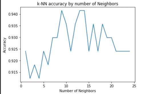
Here we can see that the accuracy of the model start decreasing as we increase the k value.
Select the best K Value for the Model
Selecting the best hyperparameter is critical to selecting the best model.
The plot above is great, but should you choose 8 or 13, or even bigger n_neighbors values?
Using GridSearchCV from the model_selection module, you can check the best parameter for your model.
import numpy as np
from sklearn.model_selection import GridSearchCV

param_grid = {'n_neighbors':np.arange(1, 50)}
knn_cv = GridSearchCV(knn, param_grid, cv=5)
knn_cv.fit(X_train, y_train)
print(knn_cv.best_params_)
print(knn_cv.best_score_)
The result tells you which k value to take to best fit your data. In this case, you should set n_neighbors to be 13.
{'n_neighbors': 6}
0.9498417721518987
Check the Confusion Matrix
It is possible that the accuracy is not fully representative. We will now try to see how many predictions are True and how many are False.
We will do this using:
- Confusion matrix
- Classification report
Quick reminder, in the coming plots we will plot the targets (0s and 1s) and not the target names. Remember that:
0=malignant1=benign
Confusion matrix
To plot the confusion matrix, we will use the confusion_matrix and plot_confusion_matrix methods from the sklearn.metrics module.
import matplotlib.pyplot as plt
from sklearn.metrics import confusion_matrix, plot_confusion_matrix

cm = confusion_matrix(y_test,y_pred)
print(cm)

color = 'white'
matrix = plot_confusion_matrix(knn, X_test, y_test, cmap=plt.cm.Blues)
matrix.ax_.set_title('Confusion Matrix', color=color)
plt.xlabel('Predicted Label', color=color)
plt.ylabel('True Label', color=color)
plt.gcf().axes[0].tick_params(colors=color)
plt.gcf().axes[1].tick_params(colors=color)
plt.show()
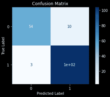
If you don’t know how to interpret this, just read my post on the confusion matrix.
Classification Report
Let’s compute the classification report to assess the quality of the predictions.
from sklearn.metrics import classification_report

print(classification_report(y_test, y_pred))
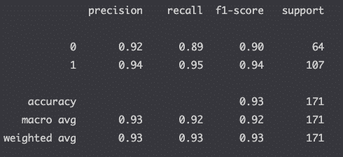
If you don’t know how to interpret this, just read my post on the classification report.
Additional Parameters for KNN
KNN allows for some flexibility providing additional parameters when training a model. For instance, along with n_neighbors, it is possible to modify the distance metrics and the weighting schemes for example.
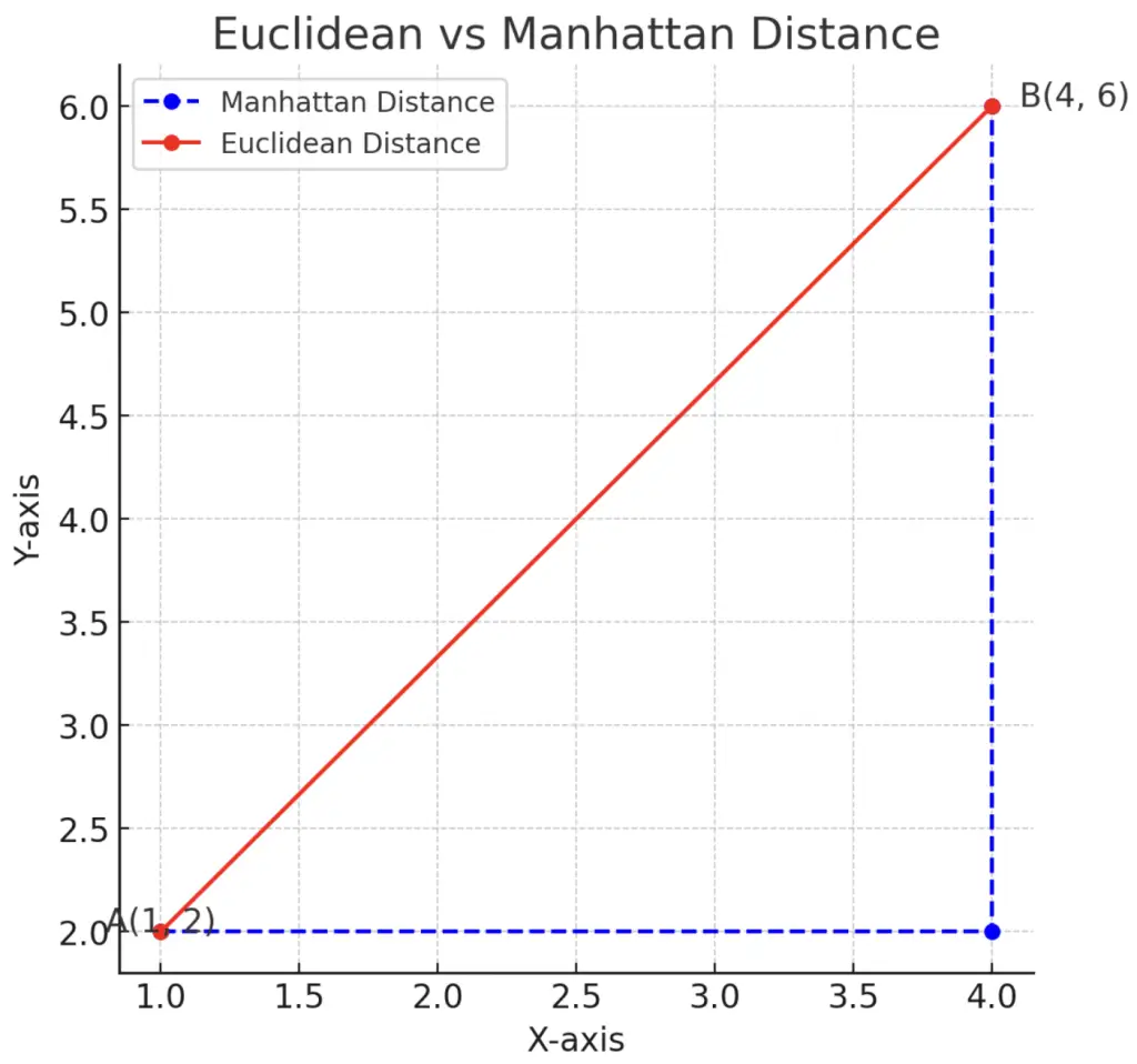
KNN Distance Metrics
By default KNN calculates the Euclidean distance between two points, but it is also possible to calculate the Manhattan distance instead.
# Example modifying the metric for KNN
KNeighborsClassifier(metric='manhattan', n_neighbors=5)
- Euclidean Distance (in read) is the straight-line distance between A and B.
- Manhattan Distance (in blue) is the sum of the horizontal and vertical distances between A and B
KNN Weighting Schemes
Weighting schemes in KNN help determine how much influence each neighbor has on a prediction. KNN allows for different weighting schemes: uniform and distance. By default KNN is uniform meaning all neighbors contribute equally to the prediction.
# Example modifying the weights metric for KNN
KNeighborsClassifier(weights='distance')
'uniform': all neighbors have equal weight. Distance from the classified data point is not important.'distance': closer neighbors have more weight than those further to the data point.
Conclusion
This project is now done. We have implemented and checked the accuracy of our k-Nearest Neighbors algorithm in Scikit-learn.

SEO Strategist at Tripadvisor, ex- Seek (Melbourne, Australia). Specialized in technical SEO. Writer in Python, Information Retrieval, SEO and machine learning. Guest author at SearchEngineJournal, SearchEngineLand and OnCrawl.