Linear Regression in Machine Learning (with Python Examples)

Linear regression in machine learning is a supervised learning approach in which computer programs try to make predictions on continuous variables.

Simply put, the goal of the linear regression algorithm is to plot a best-fit line (or curve) between dependent (target) and independent (feature/predictor) variables.

What is a Linear Regression?

Linear regression uses a straight line to compare the relationship between two variables. Other types of regressions like the logistic regression models use a curved line.

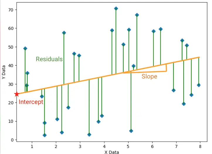
The objective of linear regression is to fit a line in a scatter plot of two continuous variables in a way that the data points lie collectively as close as possible to the line.

Linear regression is one of the several regression models used in machine learning.

Types of Linear Regression

1. Simple Linear Regression
2. Multiple Linear Regression

Simple Linear Regression

The simple linear regression is estimated using the ordinary least squares (OLS) approach.

It has a dependant and an independent variable and can be used to estimate the relationship between these two variables.

When to use the Simple Linear Regression?

1. Identify how closely related the two variables are. (e.g. ice cream sales and temperature).
2. Predict the value of the dependent variable when the independent variable changes. (e.g. the number of sales of ice cream at a given temperature).

Simple Linear Regression Model Formula

The simple linear regression model formula goes like this.

? = β₀ + β₁?₁ + ε

• ? is the dependent / target variable that we are trying to predict;
• ? is an independent variable;
• β₁ is the coefficient that quantifies the effect of ?₁ on ?.
• β₀ is the intercept of the regression line
• ε (epsilon) is the error

or the most common expression:

y = aX + b

• y is the coordinates of the dependent variable (also known as response or target variable)
• x is the coordinates of the independent variable
• a is the slope of the line
• b is the intercept where x meets y

The simple linear regression is one-way

For the simple linear regression to work:

• There must be a dependent (X) and an independent (Y) variable;
• There must be a single independent variable;
• Y must be dependent on X;
• X cannot be dependent on Y.

We could say that the sales of ice cream cones (Y) are influenced by the temperature outside (x).

However, saying that the temperature outside (Y) is influenced by the number of ice cream cones sold (X) would be a faulty assumption. In which case, the formula does not work. This is because mother nature is not dependant on Ben & Jerry’s ability to promote their products.

When two or more independent variables are used in regression analysis, the model is no longer a simple linear one. This is known as multiple regression.

Multiple Linear Regression

Multiple linear regression is similar to the simple linear regression model but has multiple independent variables that contribute to the dependent variable.

Multiple linear regression is not the same as multivariate linear regression where multiple correlated dependent variables are predicted, rather than a single scalar variable.

• multiple linear regression: y is scalar.
• multivariate linear regression: y is a vector.

Formula of the multiple linear regression

Having multiple independent variables, multiple coefficients are added to the linear function to fit each independent variable.

y = β₀ + β1?1 + β2?2 + … + βnXn + ε

• Y is the dependent variable / Target variable
• β₀ is the Intercept of the regression line
• β1, β2, …. βn are the slope of the regression lines of each feature
• X1, X2, ….Xn are the Independent / feature variables
• ε (epsilon) is the error

Make a Linear Regression in Python

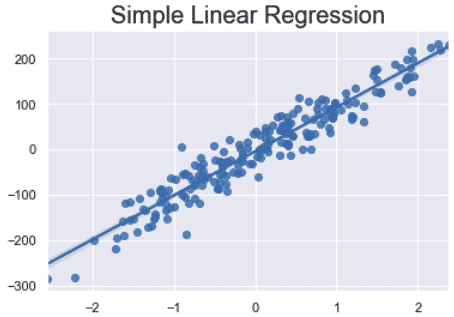
Simple linear regression using make_regression

Making a simple linear regression in Python is very easy using Scikit-learn and seaborn regplot.

import matplotlib.pyplot as plt
import seaborn as sns
from sklearn.datasets import make_regression
sns.set()

X, y = make_regression(n_samples=200, n_features=1, n_targets=1, noise=30, random_state=0)
sns.regplot(x=X, y=y)
plt.title('Simple Linear Regression', fontsize=20)
plt.show()

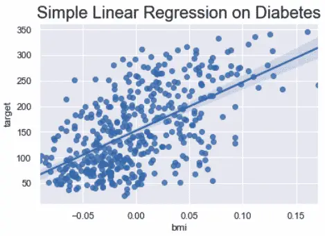
Plot simple linear regression on real-world data

You can also perform the linear regression on a real-world dataset such as the diabetes dataset.

import matplotlib.pyplot as plt
import pandas as pd 
import seaborn as sns
from sklearn.datasets import load_diabetes
sns.set() 

X, y = load_diabetes(return_X_y=True, as_frame=True)
X = X[['bmi']]

sns.regplot(x=X, y=y)
plt.title('Simple Linear Regression on Diabetes', fontsize=20)
plt.show()

Make a linear regression model

Now, using Scikit-learn, we can create a linear regression model to make a prediction on the target variable based on the input feature variables.

We will use Scikit-learn’s metrics module to evaluate the performance of the model.

from sklearn.datasets import load_diabetes
from sklearn.model_selection import train_test_split
from sklearn.linear_model import LinearRegression
from sklearn import metrics

X, y = load_diabetes(return_X_y=True, as_frame=True)
X = X[['bmi']]

X_train, X_test, y_train, y_test = train_test_split(X, y, test_size=0.3, random_state=0)

lin_reg = LinearRegression()
lin_reg.fit(X_train, y_train)

y_pred = lin_reg.predict(X_test)

print('Intercept:', lin_reg.intercept_)
print('Coefficients:', lin_reg.coef_)
print('Mean absolute error:', metrics.mean_absolute_error(y_test, y_pred))
print('Mean squared error:', metrics.mean_squared_error(y_test, y_pred))
print('Coefficient of determination (r2 Score):', metrics.r2_score(y_test, y_pred))

The result of the prediction will be something like this.

Intercept: 153.4350903922729
Coefficients: [1013.17358257]
Mean absolute error: 51.340840560752476
Mean squared error: 3921.3720274248517
Coefficient of determination (r2 Score): 0.23132831307953805

Make multiple linear regression

Making a multiple linear regression involves similar steps to making a simple linear regression.

The difference lies in the evaluation.

import matplotlib.pyplot as plt
import pandas as pd 
import seaborn as sns
from sklearn.datasets import load_diabetes
from sklearn.model_selection import train_test_split
from sklearn.linear_model import LinearRegression
from sklearn import metrics
sns.set()

X, y = load_diabetes(return_X_y=True, as_frame=True)

X_train, X_test, y_train, y_test = train_test_split(X, y, test_size=0.3, random_state=0)

lin_reg = LinearRegression()
lin_reg.fit(X_train, y_train)

y_pred = lin_reg.predict(X_test)

coef_df = pd.DataFrame(lin_reg.coef_, X.columns, columns=['Coefficient'])
coef_df.plot(kind='barh')
plt.title('Feature importance of linear regression')
plt.show()

Each feature will have a different level of influence on the predicted values. Some will influence more, some will influence less.

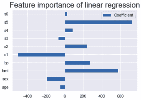
On a simple linear regression, there would be a single bar on the coefficient graph.

Understand the linear regression evaluation scores

Mean absolute error (MAE)

Absolute difference between the data and the model’s predictions

MAE = True values – Predicted values.

Mean squared error (MSE)

square of the differences between the data and the model’s predictions.

The issue with the mean absolute error is that negative difference cancels out positive differences.

Squaring these values provide a sense of the importance of the error.

For example:

(real_value_1 - pred_value_1) + (real_value_2 - pred_value_2) 
MAE = (3 - 5) + (7 - 4) = -2 + 3 = 1
MSE = (3 - 5)^2 + (7 - 4)^2 = -2^2 + 3^2 = 4 + 9 = 13

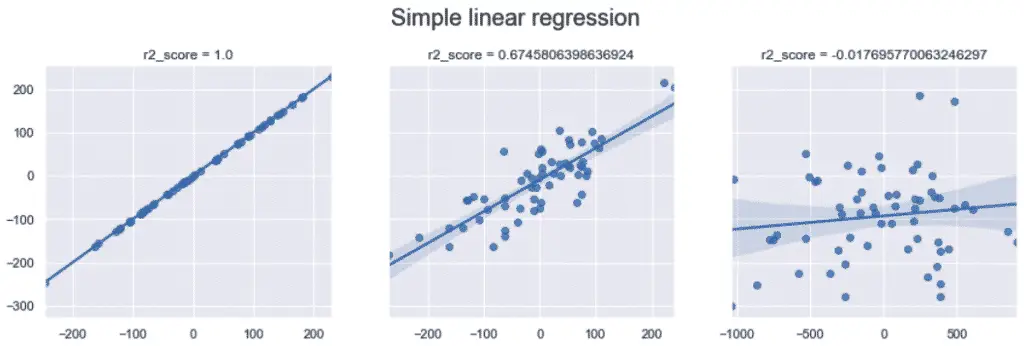
Coefficient of determination (r2 Score)

The r^2 score measures the quality of the explanation that you can get from a model. The more factors you take into consideration, the higher the r-squared will be.

R^2 = SSR / SST

• SSR: Sum of squares of the residual errors.
• SST: Total sum of the errors.

The r-squared is a measure relative to the total variability. It takes values ranging from 0 to 1.

• When R^2 = 0, the regression explains none of the variability of the data.
• When r^2 = 1, the regression explains all of the variability of the data.

Interesting Work in the Community

• Here’s how I used Python to build a regression model using an e-commerce dataset by Hülya Çoban

Conclusion

We have seen that linear regression is a statistical analysis approach for modelling the relationship between dependent and independent variables.

We also learned that linear regression performed on a single explanatory (independent) variable are called simple linear regressions; the ones performed on multiple independent variables are called multiple linear regressions.

To further your understanding, feel free to read on the linear regression estimation methods.

Jean-Christophe Chouinard

SEO Strategist at Tripadvisor, ex- Seek (Melbourne, Australia). Specialized in technical SEO. Writer in Python, Information Retrieval, SEO and machine learning. Guest author at SearchEngineJournal, SearchEngineLand and OnCrawl.