Model evaluation is used in machine learning to evaluate the performance of a model and compare different models in order to choose the best performing one. The Scikit-learn Python library provides the tool to help score and evaluate the performance of a machine learning model.
In this tutorial, we will learn how to use Sklearn to evaluate machine learning models in Python. We will use the Scikit-learn’s metrics module to evaluate the performance of a classification, a clustering and a regression problems.
Navigation
Show
How to Evaluate a Machine Learning Model in Scikit-Learn?
There are multiple techniques that can be use evaluate a machine learning model in Scikit-learn depending on the type of project and whether you are evaluation a classification, a regression or a clustering machine learning model. Here’s a general idea of the steps to perform a model evaluation:
- Load the dataset
- Split the Data
- Hyperparameter Tuning
- Train the Model
- Make Predictions
- Select a Performance Metric
- Evaluate the Model
- Plot the Confusion Matrix
- Print the Classification Report
- Plot the ROC AUC Curve
We will use the breast cancer dataset to perform a classification using K-Nearest Neighbors and then show you how to use evaluation metrics to evaluate the model.
1. Load the dataset
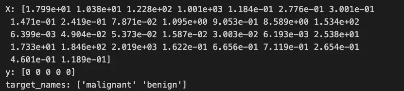
The first step is to import the dataset using the load_breast_cancer() function from the built-in Scikit-learn datasets module.
# Step 1: Load the dataset
data = load_breast_cancer()
X = data.data
y = data.target
target_names = data.target_names
print('X:',X[0],'\ny:',y[:5],'\ntarget_names:',target_names)
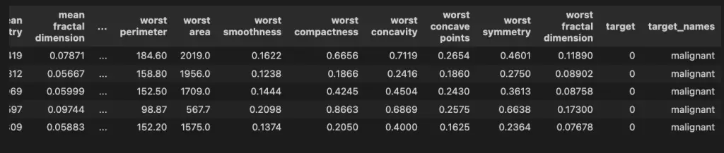
To understand the data that you are viewing, you can load the data as a Pandas DataFrame.
import pandas as pd

# Create a DataFrame from the data and target
df = pd.DataFrame(data.data, columns=data.feature_names)
df['target'] = data.target

# Optional: If you want to include the target names as well
df['target_names'] = data.target_names[df['target']]

# Print the DataFrame
df.head()
In that DataFrame, you will see that the X variable represents all the data found in the table apart from the last two columns. The target column shows the values of the y variable and the target_names columns shows values of the target_names variable. When we previewed X[0], we printed the values from the first row of data.
2. Split the Data With Train_test_split
Divide your dataset into a training set and a test set. The training set is used to train the model and the test set is used for evaluation.
from sklearn.model_selection import train_test_split

# Step 2: Split the data into training and test sets
X_train, X_test, y_train, y_test = train_test_split(X, y, test_size=0.3, random_state=42)
3. Hyperparameter Tuning
To improve the model’s performance, perform hyperparameter tuning. You can use GridSearchCV to find the best combination of hyperparameters.
# Step 3: Perform hyperparameter tuning with GridSearchCV

# Instantiate the model
knn = KNeighborsClassifier()

# Tune hyper parameters with GridSearchCV
param_grid = {"n_neighbors": [3, 5, 7, 9]}
grid_search = GridSearchCV(knn, param_grid, cv=5)
grid_search.fit(X_train, y_train)
best_k = grid_search.best_params_["n_neighbors"]
4. Train the Model
Train the machine learning model on the training data using the fit() method. Provide the best number of neighbors from previous step to the n_neighbors.
# Step 4: Train the model
knn = KNeighborsClassifier(n_neighbors=best_k)
knn.fit(X_train, y_train)
5. Make Predictions
Make predictions on the test set using the predict() method on the knn model object.
# Step 5: Make predictions
y_pred = knn.predict(X_test)
Select a Performance Metric
Choose an evaluation metric based on the type of machine learning problem, such as accuracy, precision, recall, F1 score, or area under the ROC curve (ROC AUC). The choice depends on whether you have a classification, regression, or clustering problem.
To choose the right performance metric make sure that you understand the goal of your model and choose the right metric for the type of machine learning problem. In some cases you may want precision and recall and in others a higher accuracy. You also want to select the right metric based on the type of the problem. You should use different metrics based on the type of ML problem. Here is a guideline to help you choose the right metric based on the type of machine learning problem:
- Classification: Accuracy, Precision and recall, F1-score, ROC-AUC
- Regression: Mean Squared Error, Mean Absolute Error, Root MSE (RMSE), R-squared
- Clustering: Adjusted Rand Index, Mutual Information
Check our guide explaining all of Scikit-learn’s metrics.
Evaluate the Model
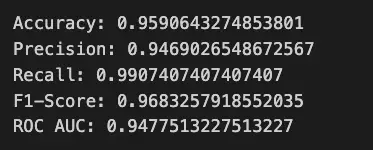
Compare the predicted labels with the true labels from the validation set or test set. Calculate the chosen performance metric using appropriate functions like accuracy_score(), precision_score(), recall_score(), f1_score(), or roc_auc_score().
from sklearn.metrics import (
    accuracy_score,
    precision_score,
    recall_score,
    f1_score,
    roc_auc_score
)

# Step 6: Evaluate the model
accuracy = accuracy_score(y_test, y_pred)
precision = precision_score(y_test, y_pred)
recall = recall_score(y_test, y_pred)
f1 = f1_score(y_test, y_pred)
roc_auc = roc_auc_score(y_test, y_pred)

print(f'Accuracy: {accuracy}')
print(f'Precision: {precision}')
print(f'Recall: {recall}')
print(f'F1-Score: {f1}')
print(f'ROC AUC: {roc_auc}')
Plot Confusion Matrix
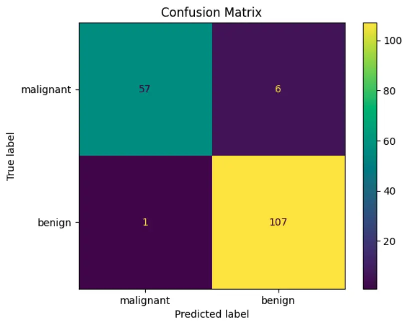
We will evaluate the model using Scikit-learn’s metrics module. From that module, we will use the confusion_matrix() function and the ConfusionMatrixDisplay() class to show and plot the confusion matrix in Python.
from sklearn.metrics import confusion_matrix, ConfusionMatrixDisplay

# Step 6: Plot the confusion matrix
cm = confusion_matrix(y_test, y_pred)
disp = ConfusionMatrixDisplay(confusion_matrix=cm, display_labels=target_names)
disp.plot()
disp.ax_.set(title='Confusion Matrix')
plt.show()
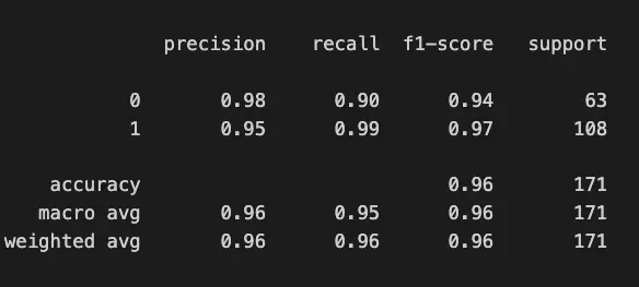
Print Classification Report
Next, we will evaluate the model’s metrics using the classification report using sklearn.metrics.classification_report.
from sklearn.metrics import classification_report

# Step 7: View the Classification Report
print(classification_report(y_test, y_pred))
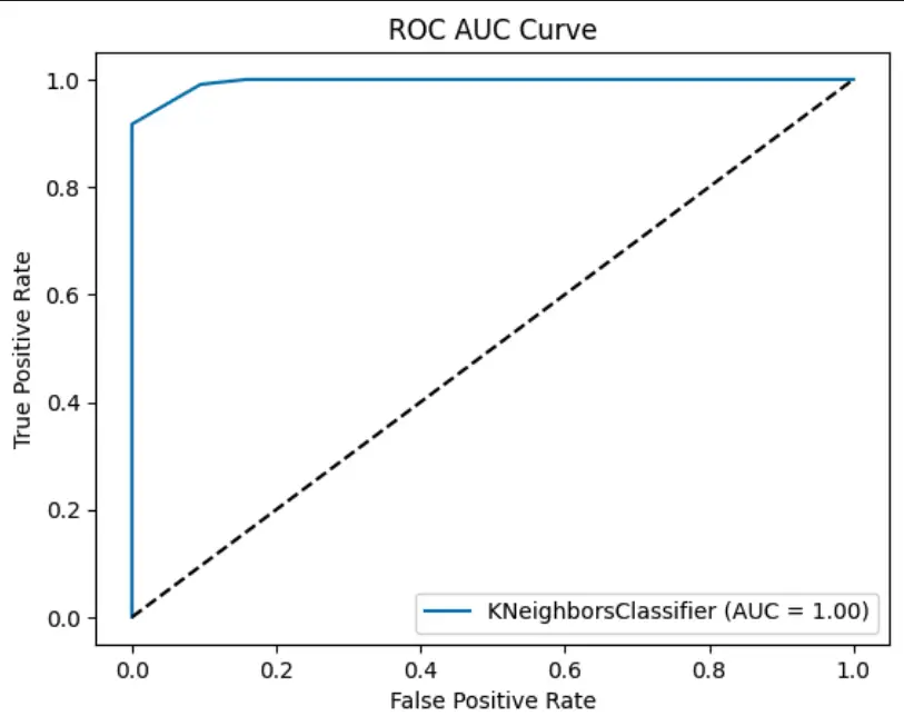
Plot the ROC AUC Curve
After, we will evaluate the False positive rates and True positive rates by plotting the ROC AUC curve using the RocCurveDisplay class of sklearn.metrics. This will show the roc_auc_score() at different classification thresholds.
import matplotlib.pyplot as plt
from sklearn.metrics import RocCurveDisplay

# Step 8: Plot the ROC AUC curve
y_scores = knn.predict_proba(X_test)
roc_display = RocCurveDisplay.from_estimator(knn, X_test, y_test)
plt.plot([0, 1], [0, 1], 'k--')
plt.xlabel('False Positive Rate')
plt.ylabel('True Positive Rate')
plt.title('ROC AUC Curve')
plt.show()
Classification Model Evaluation with Scikit-Learn
Let’s try to evaluate the performance of a machine learning model in classification problems use one of the following scoring functions from sklearn.metrics:
- accuracy_score(),
- precision_score(),
- recall_score(),
- f1_score(),
- roc_auc_score()
import matplotlib.pyplot as plt
from sklearn.datasets import load_breast_cancer
from sklearn.model_selection import train_test_split, GridSearchCV
from sklearn.neighbors import KNeighborsClassifier
from sklearn.metrics import (
    confusion_matrix,
    ConfusionMatrixDisplay,
    classification_report,
    accuracy_score,
    precision_score,
    recall_score,
    f1_score,
    roc_auc_score,
    RocCurveDisplay
)

# Step 1: Load the dataset
data = load_breast_cancer()
X = data.data
y = data.target
target_names = data.target_names


# Step 2: Split the data into training and test sets
X_train, X_test, y_train, y_test = train_test_split(X, y, test_size=0.3, random_state=42)

# Step 3: Perform hyperparameter tuning with GridSearchCV

# Instantiate the model to be tuned
knn = KNeighborsClassifier()

# Tune hyper parameters with GridSearchCV
param_grid = {"n_neighbors": [3, 5, 7, 9]}
grid_search = GridSearchCV(knn, param_grid, cv=5)
grid_search.fit(X_train, y_train)
best_k = grid_search.best_params_["n_neighbors"]

# Step 4: Train the model
knn = KNeighborsClassifier(n_neighbors=best_k)
knn.fit(X_train, y_train)

# Step 5: Make predictions
y_pred = knn.predict(X_test)

# Step 6: Evaluate the model
accuracy = accuracy_score(y_test, y_pred)
precision = precision_score(y_test, y_pred)
recall = recall_score(y_test, y_pred)
f1 = f1_score(y_test, y_pred)
roc_auc = roc_auc_score(y_test, y_pred)

print(f'Accuracy: {accuracy}')
print(f'Precision: {precision}')
print(f'Recall: {recall}')
print(f'F1-Score: {f1}')
print(f'ROC AUC: {roc_auc}')

# Step 6: Plot the confusion matrix
cm = confusion_matrix(y_test, y_pred)
disp = ConfusionMatrixDisplay(confusion_matrix=cm, display_labels=target_names)
disp.plot()
disp.ax_.set(title='Confusion Matrix')
plt.show()

# Step 7: View the Classification Report
print(classification_report(y_test, y_pred))

# Step 8: Plot the ROC AUC curve
y_scores = knn.predict_proba(X_test)
roc_display = RocCurveDisplay.from_estimator(knn, X_test, y_test)
plt.plot([0, 1], [0, 1], 'k--')
plt.xlabel('False Positive Rate')
plt.ylabel('True Positive Rate')
plt.title('ROC AUC Curve')
plt.show()
Regression Model Evaluation with Scikit-Learn
Let’s try to evaluate the performance of a machine learning model in regression problems, use one of the following scoring functions from sklearn.metrics:
- mean_absolute_error(),
- mean_squared_error(),
- r2_score()
import matplotlib.pyplot as plt
from sklearn.datasets import load_diabetes
from sklearn.model_selection import train_test_split, GridSearchCV
from sklearn.neighbors import KNeighborsRegressor
from sklearn.metrics import (
mean_squared_error,
mean_absolute_error,
r2_score,
)
# Step 1: Load the dataset
data = load_diabetes()
X = data.data
y = data.target
# Step 2: Split the data into training and test sets
X_train, X_test, y_train, y_test = train_test_split(X, y, test_size=0.3, random_state=42)
# Step 3: Perform hyperparameter tuning with GridSearchCV
# Instantiate the model to be tuned
knn = KNeighborsRegressor()
# Tune hyperparameters with GridSearchCV
param_grid = {"n_neighbors": [3, 5, 7, 9]}
grid_search = GridSearchCV(knn, param_grid, cv=5)
grid_search.fit(X_train, y_train)
best_k = grid_search.best_params_["n_neighbors"]
# Step 4: Train the model
knn = KNeighborsRegressor(n_neighbors=best_k)
knn.fit(X_train, y_train)
# Step 5: Make predictions
y_pred = knn.predict(X_test)
# Step 6: Evaluate the model
mse = mean_squared_error(y_test, y_pred)
mae = mean_absolute_error(y_test, y_pred)
r2 = r2_score(y_test, y_pred)
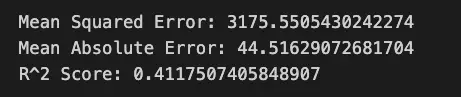
print(f'Mean Squared Error: {mse}')
print(f'Mean Absolute Error: {mae}')
print(f'R^2 Score: {r2}')
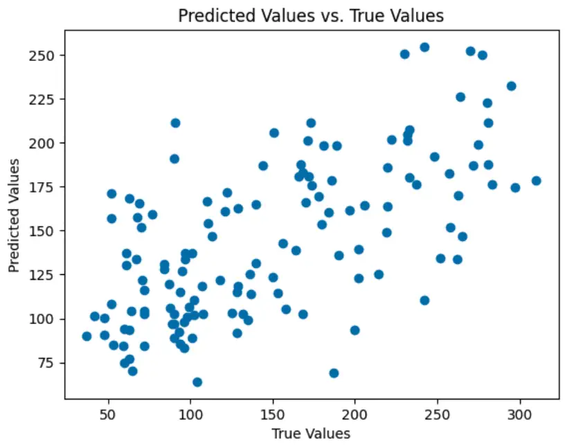
# Step 7: Plot the predicted values vs. true values
plt.scatter(y_test, y_pred)
plt.xlabel('True Values')
plt.ylabel('Predicted Values')
plt.title('Predicted Values vs. True Values')
plt.show()
Clustering Model Evaluation with Scikit-Learn
Let’s try to evaluate the performance of a machine learning model in clustering problems, use one of the following scoring functions from sklearn.metrics:
- silhouette_score(),
- calinski_harabasz_score(),
- davies_bouldin_score()
import matplotlib.pyplot as plt
from sklearn.datasets import load_iris
from sklearn.model_selection import train_test_split, GridSearchCV
from sklearn.cluster import KMeans
from sklearn.metrics import (
silhouette_score,
calinski_harabasz_score,
davies_bouldin_score
)
# Step 1: Load the dataset
data = load_iris()
X = data.data
# Step 2: Split the data into training and test sets (not used in clustering)
X_train, X_test = train_test_split(X, test_size=0.3, random_state=42)
# Step 3: Perform hyperparameter tuning with GridSearchCV
# Instantiate the model to be tuned
kmeans = KMeans()
# Tune hyperparameters with GridSearchCV
param_grid = {"n_clusters": [2, 3, 4, 5]}
grid_search = GridSearchCV(kmeans, param_grid, cv=5)
grid_search.fit(X)
# Step 4: Train the model with the best hyperparameters
best_k = grid_search.best_params_["n_clusters"]
kmeans = KMeans(n_clusters=best_k)
kmeans.fit(X)
# Step 5: Make predictions (labels) for the entire dataset
labels = kmeans.predict(X)
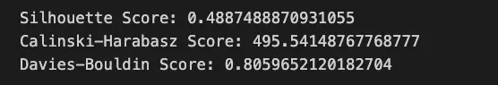
# Step 6: Evaluate the model
silhouette = silhouette_score(X, labels)
calinski_harabasz = calinski_harabasz_score(X, labels)
davies_bouldin = davies_bouldin_score(X, labels)
print(f'Silhouette Score: {silhouette}')
print(f'Calinski-Harabasz Score: {calinski_harabasz}')
print(f'Davies-Bouldin Score: {davies_bouldin}')
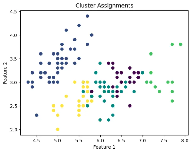
# Step 7: Plot the cluster assignments
plt.scatter(X[:, 0], X[:, 1], c=labels)
plt.xlabel('Feature 1')
plt.ylabel('Feature 2')
plt.title('Cluster Assignments')
plt.show()
Conclusion
This is the end of this tutorial on machine learning model evaluation with Scikit-learn and Python. For more detail check out the Scikit-learn’s documentation on model evaluation.

SEO Strategist at Tripadvisor, ex- Seek (Melbourne, Australia). Specialized in technical SEO. Writer in Python, Information Retrieval, SEO and machine learning. Guest author at SearchEngineJournal, SearchEngineLand and OnCrawl.