Classification Machine Learning Project in Scikit-Learn (Python Example)

In this article, we will use Python to learn Scikit-learn through a typical machine learning classification problem.

We will:

Load the dataset
Explore the dataset
Split data into features and targets (independent and dependent variables)
Create new features (feature engineering)
Preprocess the data
Split data into training and testing datasets
Run the classification algorithm and find their ideal hyperparameter
Train the model
Evaluate each model

Load the Titanic dataset with Scikit-learn

Most machine learning models need preprocessing of untidy data.

The Titanic dataset is a great one to use to practice machine learning classification.

We will load the data using the fetch_openml method available with the scikit-learn library.

from sklearn.datasets import fetch_openml

# load dataset
titanic = fetch_openml('titanic', version=1, as_frame=True)
df = titanic['data']
df['survived'] = titanic['target']

Exploratory data analysis

Exploratory data analysis (EDA) is an important step of the machine learning process.

It helps understand, clean and validate what data is important, missing or in the wrong format for your machine learning model to understand.

Load Packages for exploratory data analysis

To perform EDA, we will use Matplotlib, Pandas and Seaborn.

import matplotlib.pyplot as plt
import pandas as pd 
import seaborn as sns

from sklearn.datasets import fetch_openml
sns.set()

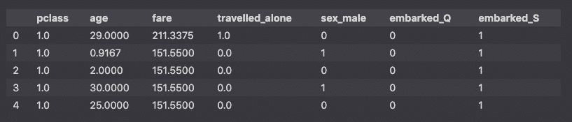
Preview the dataset

Let’s start by understanding our dataset.

df.head(3)

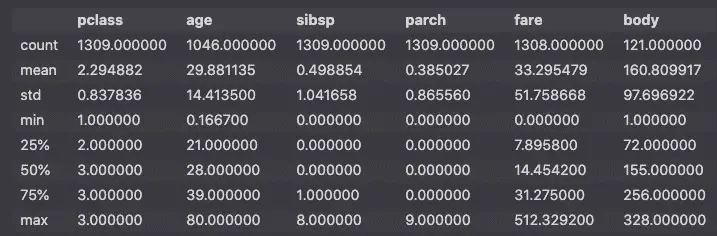
Generate descriptive statistics

Preview the numeric features descriptive statistics.

df.describe()

Here you can see great variation in how the data is spread by looking at the `std`.

Show null columns

df.info()

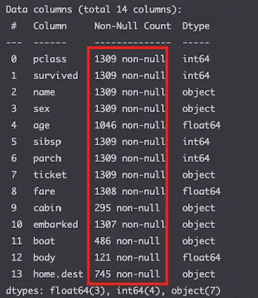
All columns have value in them.

Show missing values

df.isnull().sum()

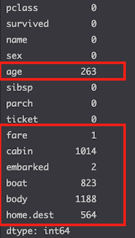
A lot of columns are missing values.

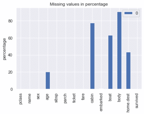
Let’s visualize that.

miss_vals = pd.DataFrame(df.isnull().sum() / len(df) * 100)
miss_vals.plot(kind='bar',
    title='Missing values in percentage',
    ylabel='percentage'
    )

plt.show()

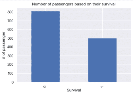
Visualize the target variable

Since we will try to predict survival, let’s visualize the survival column.

df.survived.value_counts().plot(kind='bar')

plt.xlabel('Survival')
plt.ylabel('# of passengers')
plt.title('Number of passengers based on their survival')
plt.show()

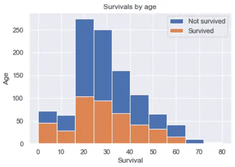
Survival by age

fig, ax = plt.subplots()

ax.hist(df.age.dropna(), label='Not survived')
ax.hist(df['age'][df.survived == '1'].dropna(), label='Survived')

plt.xlabel('Survival')
plt.ylabel('Age')
plt.title('Survivals by age')
plt.legend()
plt.show()

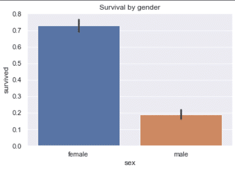
Survival by gender

df['survived'] = df.survived.astype('int')

sns.barplot(
    x='sex',
    y='survived',
    data=df
)

plt.title('Survival by gender')
plt.show()

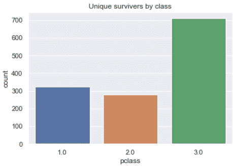
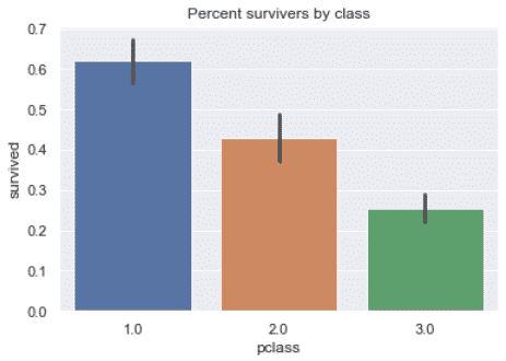
Survivers by class

sns.countplot(x='pclass', data=df)
plt.title('Unique survivers by class')
plt.show()

sns.barplot(x='pclass', y='survived', data=df)
plt.title('Percent survivers by class')
plt.show()

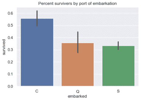
Survivers by port of embarkation

sns.barplot(x='embarked', y='survived', data=df)
plt.title('Percent survivers by port of embarkation')
plt.show()

Initiate Independent and Dependent variables

Classification algorithms will try to classify targets (dependent variables) using the features (independent variables) as predictors.

Here, the column that we want to make a prediction on is the column that states whether or not the passenger survived.

We can assign the features to X by using the drop method to keep all columns except the target and assigning the target to y.

from sklearn.datasets import fetch_openml

# load dataset
titanic = fetch_openml('titanic', version=1, as_frame=True)
df = titanic['data']
df['survived'] = titanic['target']

# Assign Dependent and Independent variables
X = df.drop('survived', axis=1)
y = df['survived']

Better still, fetch_openml() does that for you with the return_X_y keyword.

from sklearn.datasets import fetch_openml

X, y = fetch_openml('titanic', version=1, as_frame=True, return_X_y=True)

Feature Engineering

Some features don’t have much meaning when used alone. However, we can give them meaning by looking at the context.

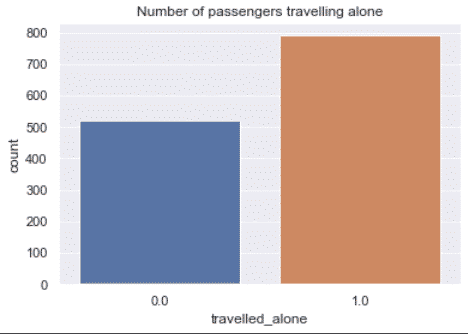
For example, the sibsp and parch columns tell you if the passenger was travelling with siblings, parents or children. By combining these features, you can infer if the passenger was travelling alone, and see if that impacted the chances of survival.

X['family'] = X['sibsp'] + X['parch']
X.loc[X['family'] > 0, 'travelled_alone'] = 0
X.loc[X['family'] == 0, 'travelled_alone'] = 1
X.drop(['family', 'sibsp', 'parch'], axis=1, inplace=True)
sns.countplot(x='travelled_alone', data=X)
plt.title('Number of passengers travelling alone')
plt.show()

Preprocess Data with Scikit-learn

There are two main reasons why you want to do data preprocessing before training your machine learning model:

To satisfy the requirements of the scikit-learn api
To clean erroneous and missing data from datasets

We will:

Remove features that we don’t want
Fill missing values
Convert categorical data features to numeric format
Scale numeric features

Remove features that we don’t want

First, we remove the columns that have too many missing values.

# remove high missing value columns
X.drop(['cabin', 'boat', 'body'], axis=1, inplace=True)

# remove less interesting features
X.drop(['name','ticket','home.dest'], axis=1, inplace=True)

Fill Missing Values (Imputation)

To use Scikit-learn, you should have no missing values in your dataset.

Thus, using SimpleImputer, we will fill the missing values using the mean for numeric data, and the most_frequent value for categorical data.

from sklearn.impute import SimpleImputer

def get_parameters(df):
    parameters = {}
    for col in df.columns[df.isnull().any()]:
        if df[col].dtype == 'float64' or df[col].dtype == 'int64' or df[col].dtype =='int32':
            strategy = 'mean'
        else:
            strategy = 'most_frequent'
        missing_values = df[col][df[col].isnull()].values[0]
        parameters[col] = {'missing_values':missing_values, 'strategy':strategy}
    return parameters

parameters = get_parameters(X)

for col, param in parameters.items():
    missing_values = param['missing_values']
    strategy = param['strategy']
    imp = SimpleImputer(missing_values=missing_values, strategy=strategy)
    X[col] = imp.fit_transform(X[[col]])

X.isnull().sum()

Handle Categorical Data

Scikit learn requires categorical data to be converted into continuous numeric format. Using the pandas get_dummies method, we will convert categorical features into 0s and 1s.

# handle categorical data
cat_cols = X.select_dtypes(include=['object','category']).columns
dummies = pd.get_dummies(X[cat_cols], drop_first=True)
X[dummies.columns] = dummies
X.drop(cat_cols, axis=1, inplace=True)
X.head()

Scale Numeric Data

To improve model performance, we will scale the numeric features so that they all have a mean=0 and a standard deviation = 1.

# Scale numeric data
from sklearn.preprocessing import StandardScaler

# Select numerical columns
num_cols = X.select_dtypes(include=['int64', 'float64', 'int32']).columns

# Apply StandardScaler
scaler = StandardScaler()
X[num_cols] = scaler.fit_transform(X[num_cols])

Split into Training and Testing Sets

We could apply the machine learning model to the entire dataset, but that wouldn’t be useful to evaluate the model performance. Instead, we split the dataset into training and testing datasets.

from sklearn.model_selection import train_test_split

RAND_STATE = 42

X_train, X_test, y_train, y_test = train_test_split(X, y, test_size=0.3, random_state=RAND_STATE)

Then, we will apply the model to the training set, and compare the result to the actual data in the test set.

Choose the best classifier algorithm

There are many classification machine learning models in Scikit-learn.

We will need to compare them and choose the best model to predict the data.

The models that we will look at are:

LogisticRegression
KNeighborsClassifier
SVC
RandomForestClassifier
DecisionTreeClassifier

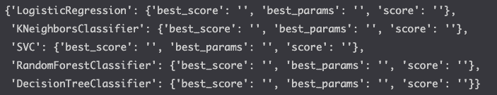
Create a dictionary to store results

cross_val_scores = {}

models = [
    'LogisticRegression', 
    'KNeighborsClassifier',
    'SVC',
    'RandomForestClassifier',
    'DecisionTreeClassifier'
    ]

empty_dict = {
    'best_score':'',
    'best_params':'',
    'score':''
    }

for m in models:
    cross_val_scores[m] = empty_dict

cross_val_scores

LogisticRegression

Create a logistic regression with the LogisticRegression algorithm.

Below, you will see that we will execute the hyperparameter tuning for each of the models using GridSearchCV. This will allow us not only to compare the models, but to identify the best parameters for each model.

%%time
from sklearn.linear_model import LogisticRegression
from sklearn.model_selection import GridSearchCV

params = {
    'C': [0.001, 0.01, 0.1, 1.],
    'penalty': ['l1', 'l2']
}

log_reg = LogisticRegression(
    random_state=RAND_STATE, 
    class_weight='balanced',
    solver='liblinear'
    )

log_reg_cv = GridSearchCV(
    log_reg, 
    param_grid=params, 
    cv=5,
    scoring='accuracy',
)

log_reg_cv.fit(X_train, y_train)

cross_val_scores['LogisticRegression']['best_score'] = log_reg_cv.best_score_
cross_val_scores['LogisticRegression']['best_params'] = log_reg_cv.best_params_
cross_val_scores['LogisticRegression']['score'] = log_reg_cv.score(X_test, y_test)

KNeighborsClassifer

Create the classification using the K-Nearest neighbors algorithm.

%%time
import numpy as np 

from sklearn.neighbors import KNeighborsClassifier
from sklearn.model_selection import GridSearchCV

params = {'n_neighbors': np.arange(1, 50)}

knn = KNeighborsClassifier()

knn_cv = GridSearchCV(
    knn, 
    param_grid=params,
    cv=5,
    scoring='accuracy'
    )

knn_cv.fit(X_train, y_train)

cross_val_scores['KNeighborsClassifier']['best_score'] = knn_cv.best_score_
cross_val_scores['KNeighborsClassifier']['best_params'] = knn_cv.best_params_
cross_val_scores['KNeighborsClassifier']['score'] = knn_cv.score(X_test, y_test)

SVC

Create the classification using the SVC algorithm.

%%time
from sklearn.svm import SVC
from sklearn.model_selection import GridSearchCV

params = {
    'C': [0.001, 0.01, 0.1, 1.],
    'kernel': ['linear', 'poly', 'rbf', 'sigmoid'],
    'gamma': ['scale', 'auto'],
}

svc = SVC(
    random_state=RAND_STATE,
    class_weight='balanced',
    probability=True,
)

svc_cv = GridSearchCV(
    svc, 
    param_grid=params, 
    cv=5,
    scoring='accuracy',
)

svc_cv.fit(X_train, y_train)

cross_val_scores['SVC']['best_score'] = svc_cv.best_score_
cross_val_scores['SVC']['best_params'] = svc_cv.best_params_
cross_val_scores['SVC']['score'] = svc_cv.score(X_test, y_test)

RandomForestClassifier

Create the classification using the popular ensemble learning algorithm: the RandomForestClassifier.

%%time
from sklearn.ensemble import RandomForestClassifier
from sklearn.model_selection import GridSearchCV

params = {
    'n_estimators': [5, 10, 15, 20, 25], 
    'max_depth': [3, 5, 7, 9, 11, 13],
}
rand_forest = RandomForestClassifier(
    random_state=RAND_STATE,
    class_weight='balanced',
)

rf_cv = GridSearchCV(
    rand_forest, 
    param_grid=params, 
    cv=5,
    scoring='accuracy',
)

rf_cv.fit(X_train, y_train)

cross_val_scores['RandomForestClassifier']['best_score'] = rf_cv.best_score_
cross_val_scores['RandomForestClassifier']['best_params'] = rf_cv.best_params_
cross_val_scores['RandomForestClassifier']['score'] = rf_cv.score(X_test, y_test)

DecisionTree

Create the classification using the DecisionTreeClassifier algorithm.

%%time
from sklearn.tree import DecisionTreeClassifier
from sklearn.model_selection import GridSearchCV

params = {
    'max_depth': [3, 5, 7, 9, 11, 13],
}

decision_tree = DecisionTreeClassifier(
    random_state=RAND_STATE,
    class_weight='balanced',
)

dt_cv = GridSearchCV(
    decision_tree, 
    param_grid=params, 
    cv=5,
    scoring='accuracy',
)

dt_cv.fit(X_train, y_train)

cross_val_scores['DecisionTreeClassifier']['best_score'] = dt_cv.best_score_
cross_val_scores['DecisionTreeClassifier']['best_params'] = dt_cv.best_params_
cross_val_scores['DecisionTreeClassifier']['score'] = dt_cv.score(X_test, y_test)

Compare the Results

Now, let’s compare the machine learning classification algorithms against each other.

pd.DataFrame(cross_val_scores).T.sort_values(by='best_score',ascending=False)

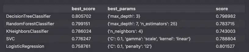
This report tells me that the best algorithm to choose in this case is the DecisionTreeClassifier with the max_depth parameter set to 3.

Build the model into a Pipeline

Let’s put everything together by building a Pipeline to run each of these steps together.

import pandas as pd 
import matplotlib.pyplot as plt

from sklearn.datasets import fetch_openml
from sklearn.compose import ColumnTransformer
from sklearn.impute import SimpleImputer
from sklearn.tree import DecisionTreeClassifier
from sklearn.metrics import classification_report, plot_confusion_matrix
from sklearn.model_selection import train_test_split
from sklearn.pipeline import Pipeline
from sklearn.preprocessing import OneHotEncoder, StandardScaler

# Set random state for reproducibility
RAND_STATE = 42

# load data
X, y = fetch_openml('titanic', version=1, as_frame=True, return_X_y=True)

# preprocessing
X['family'] = X['sibsp'] + X['parch']
X.loc[X['family'] > 0, 'travelled_alone'] = 0
X.loc[X['family'] == 0, 'travelled_alone'] = 1
X.drop(['family', 'sibsp', 'parch'], axis=1, inplace=True)
X.drop(['cabin', 'boat', 'body'], axis=1, inplace=True)
X.drop(['name','ticket','home.dest'], axis=1, inplace=True)

# handle numeric features
numeric_features = ['age','fare']
numeric_transformer = Pipeline(steps=[
    ('imputer', SimpleImputer(strategy='mean')),
    ('scaler', StandardScaler())])

# handle categorical features
categorical_features = ['embarked', 'sex', 'pclass', 'travelled_alone']
categorical_transformer = Pipeline(steps=[
    ('imputer', SimpleImputer(strategy='most_frequent')),
    ('scaler', OneHotEncoder(handle_unknown='ignore'))])

# Create a transformer
preprocessor = ColumnTransformer(
    transformers=[
        ('num', numeric_transformer, numeric_features),
        ('cat', categorical_transformer, categorical_features)])

# Run the classifier
classifier = DecisionTreeClassifier(
    random_state=RAND_STATE,
    class_weight='balanced',
    max_depth=3
    )
  
# Split into training and testing 
X_train, X_test, y_train, y_test = train_test_split(X, y, test_size=0.3, random_state=RAND_STATE)

# Set the Pipeline
model = Pipeline(steps=[('preprocessor', preprocessor),
                      ('classifier', classifier)])

# Fit the pipeline
model.fit(X_train, y_train)

# Predict
y_pred = model.predict(X_test)

# Evaluate
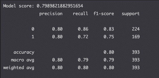
print(f'Model score: {model.score(X_test, y_test)}')

# compute the classification report
print(classification_report(y_test, y_pred))

This is it. You can see that the model score is the same as what we computed earlier.

We also used Scikit-learn’s metrics module to compute the classification report to evaluate each model.

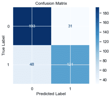
Now, we’ll plot the confusion matrix to look at true-positive and false-positive rates.

from sklearn.metrics import classification_report, plot_confusion_matrix
# plot confusion matrix
color = 'black'
matrix = plot_confusion_matrix(model, X_test, y_test, cmap=plt.cm.Blues)
matrix.ax_.set_title('Confusion Matrix', color=color)
plt.xlabel('Predicted Label', color=color)
plt.ylabel('True Label', color=color)
plt.gcf().axes[0].tick_params(colors=color)
plt.gcf().axes[1].tick_params(colors=color)
plt.show()

Feature Importance

Let’s look at which features influence the model the most.

%%time
from sklearn.tree import DecisionTreeClassifier
from sklearn.model_selection import GridSearchCV

print(cross_val_scores['DecisionTreeClassifier']['best_params'])

decision_tree = DecisionTreeClassifier(
    random_state=RAND_STATE,
    class_weight='balanced',
    max_depth=3
)


decision_tree.fit(X_train, y_train)

feature_imp = decision_tree.feature_importances_

labels = list(X_train.columns)
plt.barh([x for x in range(len(feature_imp))], feature_imp)
plt.title('DecisionTreeClassifier Feature Importance')
plt.yticks(range(len(labels)), labels)
plt.show()

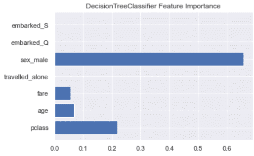
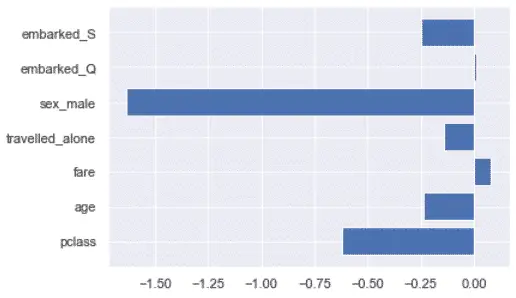
Above, we can see that we could potentially get rid of the port of embarkation and the travelled alone features since they don’t seem to impact the results DecisionTreeClassifier algorithm.

Beware, that wouldn’t be true for any algorithm.

For example, the port of embarkation has some impact on the LogisticRegression algorithm.

Conclusion

Wow. This was a lot.

We compared the most popular classification machine learning algorithms in Scikit learn against the Titanic dataset.

5/5 - (2 votes)

Jean-Christophe Chouinard

SEO Strategist at Tripadvisor, ex- Seek (Melbourne, Australia). Specialized in technical SEO. Writer in Python, Information Retrieval, SEO and machine learning. Guest author at SearchEngineJournal, SearchEngineLand and OnCrawl.