In this project, we will learn how to use Python to cluster URLs from Google Search Console by analysing the queries that each page ranks for in Google. We will use KMeans and TF-IDF to identify category groupings and potential duplicated pages.
This tutorial is Part-3 of a series on using unsupervised learning for the clustering of web pages.
- Extract Google Search Console Queries by Page (using a python Wrapper)
- TF-IDF on Google Search Console Data
- Clustering and De-duplication of web pages using KMeans and TF-IDF
First, we will create groupings and show the most common bigrams for each cluster to help define the category label.
Second, we will identify potential duplicated pages.
We will rely on Scikit-learn and NLTK for this tutorial. The machine learning algorithms covered are:
- TF-IDF: to create word vectors for each page’s queries
- KMeans: for the clustering of the pages.
- PCA: for the dimensionality reduction of the features
- NLTK: for the tokenization of the queries.
Navigation
Show
Getting Started
For this tutorial, you will also need to install Python and install the following libraries from your command prompt or Terminal.
$ pip install scikit-learn
You will also need to install NLTK.
Overview of the Dataset
In the following tutorial, I am using a TF-IDF word vector of Google Search Console queries by pages that we created in the last post of this series.
There are three 3 variables that are already available at the start of this project.
X: a TF-IDF sparse matrixtfidf_df: a tf-idf dataframequeries: a list of strings containing all the queries for each page
We will have a look at each variable for those who want to follow along without replicating the code. For those interested in replicating the code, you will need to start with the first post of the series.
Let’s look at the tf-idf sparse matrix stored in X.
print(X)
  (0, 4815)	0.00924015693268128
  (0, 4794)	0.00924015693268128
  (0, 4783)	0.010652867898559805
  (...)	...
(135, 2296)	0.01343220744505455
In a digestible format, the data we start with is essentially a dataset where:
- rows are the pages from Google Search Console,
- columns are the unique words (ngrams) of all the queries that lead to a site from Google,
- values are the tf-idf score of each word relative to each page
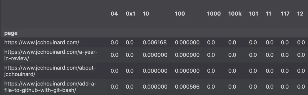
Looking at the shape of the dataframe, we see that the dataset has 135 articles and 4831 relevant individual words leading to it from Google.
tfidf_df.shape
#(135, 4837)
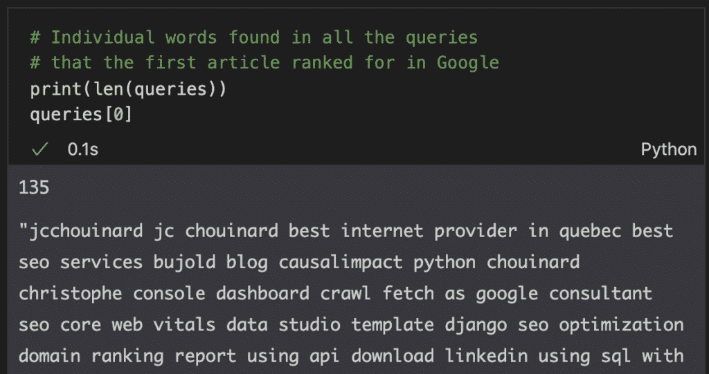
We also have a list called queries that contain 136 elements.
Each element represents a large string with each of the individual words for which the page ranked in Google, separated by a space. The 0 index represents the first page’s queries.
Part 1. Create category clusters of web pages using KMeans
KMeans requires you to define the number of clusters that you want to end up with.
Defining the number of clusters will depend on the number of pages on your site.
Here, with 135 articles, I believe I will need around 15-20 categories to describe all the articles.
This isn’t super scientific, but we’ll see more advanced techniques to find the optimal number of clusters when we try to identify duplicated pages later.
After a few iterations, I found that having 20 categories was producing interesting results.
from sklearn.cluster import KMeans

# define number of categories (clusters)
k = 20

# Instantiate the model
model = KMeans(
    n_clusters=k,
    init='k-means++',
    max_iter=100,
    n_init=1)

# Train the model on X
model.fit(X)
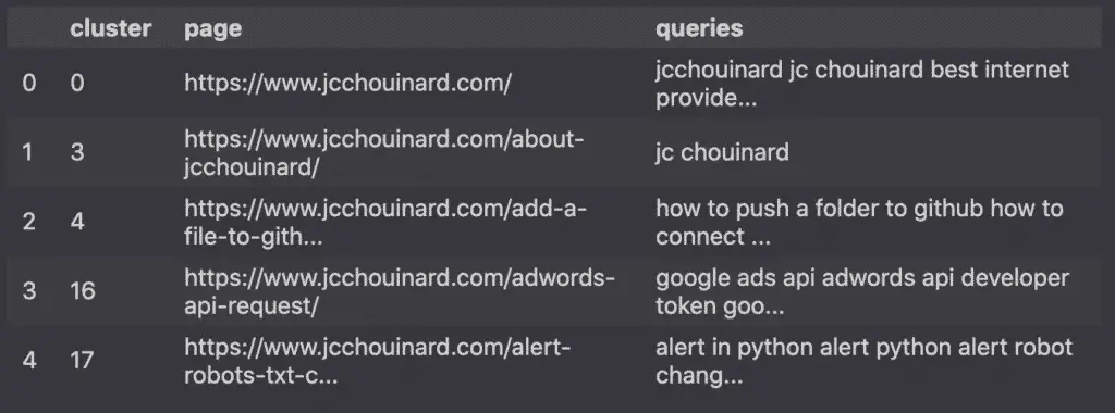
Combine the clusters to the pages and their queries
Next, we will combine the clusters generated by KMeans to the individual pages and their corresponding queries.
Then, we’ll add the result to a Pandas DataFrame.
import pandas as pd
# assign predicted clusters
labels = model.labels_

# create a dataframe that contains
# clusters matched to pages and their queries
mapping = list(zip(labels, grouped_df.index, queries))
clusters = pd.DataFrame(mapping, columns=['cluster','page','queries'])
clusters.head()
Let’s look at the distribution between clusters and plot into Seaborn.
import matplotlib.pyplot as plt
import seaborn as sns
sns.set()

clusters.cluster.value_counts().sort_index().plot(kind='bar')
plt.xlabel('clusters')
plt.ylabel('# articles')
plt.title('Number of article per cluster')
plt.show()
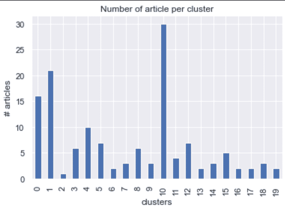
Above, we can see categories with more articles than others, but nothing too crazy showing that 20 may be a good number of clusters to describe the data.
Find most common bigrams in each cluster
Bigrams are combinations of 2 words.
python seo, seo python, seo html, keyword density, ...
What we will do is take all the individual words…
seo, python, clustering
… and permutate them against each other to create word pairs.
seo python,
python seo,
seo clustering,
clustering seo,
python clustering,
cluustering python
That permutation will be done using this function.
def find_bigrams(input_list):
    return list(zip(input_list, input_list[1:]))
We will also want to remove stopwords like “I”, “the”, “they” that can pollute the information.
The black cat
['the','black','cat']
['black', 'cat']
from nltk.corpus import stopwords

stopwords = stopwords.words('english')
Then, for each cluster we will:
- Subset the dataframe matchin the cluster
- Combine all the queries in a single string
- Remove stopwords from tokens
- Generate bigrams
- Count bigrams
- Select most common bigrams
- Store the data
from collections import Counter
from nltk.tokenize import word_tokenize

my_dict = {}
n_clusters = clusters['cluster'].unique()

# for each cluster
for c in n_clusters:
    # 1
    asset = clusters[clusters['cluster'] == c]
    asset = asset['queries']
    m_asset = ' '.join(asset)
    # 2
    tokens = word_tokenize(m_asset)
    # 3
    words = [word for word in tokens if not word in stopwords]
    # 4
    bigrams = find_bigrams(words)
    bigrams = list(map(' '.join, bigrams))
    # 5
    counts = Counter(bigrams)
    # 6
    most_common = counts.most_common(4)
    most_freq = [bigram[0] for bigram in most_common]
    # 7
    my_dict[c] = ','.join(most_freq)

my_dict
The output is a dictionary with top bigrams by cluster.
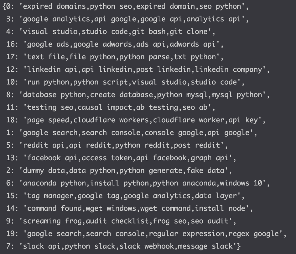
Now, I already have a sense of the categories that I will need to create:
- Group 0 seems to be a bunch of random stuff being grouped together.
- Group 12 talks about Linkedin API
- Group 18 talks about pagespeed
- all the way up to group 7 that talks about Slack api
Add the number of article per cluster
Next, we will add the number of pages for each cluster.
This will be used to provide more information on the plot.
# Add number of article per cluster
val_count = clusters['cluster'].value_counts()
for i in range(len(val_count)):
    my_dict[i] += f' ({val_count[i]})'
#before
'google analytics,api google,google api,analytics api'

#after
'google analytics,api google,google api,analytics api (6)'
Plot the Clustered Data
The upcoming steps are a little tougher to grasp.
We will try to plot our clusters on a graph and show the cluster centroids chosen by KMeans.
Dimension reduction
We need to perform dimensionality reduction to the data to reduce the risk of overfitting the model to noisy features. Dimension reduction will be done through Principal component analysis (PCA) using this solution from Stackoverflow.
from sklearn.decomposition import PCA

# Dimensionality reduction
# Reduce features to 2D
pca = PCA(n_components=2)
reduced_features = pca.fit_transform(X.toarray())

# Reduce centroids to 2D
reduced_centroids = pca.transform(model.cluster_centers_)

print('Tf-IDF feature size: ', X.toarray().shape)
print('PCA feature size: ', reduced_features.shape)
print('Tf-IDF cluster centroids size: ', model.cluster_centers_.shape)
print('PCA centroids size: ', reduced_centroids.shape)
The printed result shows the 2-dimensional dataset that we will use to plot into a graph:
Tf-IDF feature size:  (135, 4837)
PCA feature size:  (135, 2)
Tf-IDF cluster centroids size:  (20, 4837)
PCA centroids size:  (20, 2)
Predict the cluster of each page
Next, we will use the model that we trained earlier to predict the clusters for each page.
# predict the labels groupings
predictions = model.predict(X)
predictions
The result is an array with one value per page on the site.
array([ 0,  3,  4, 16, 17, 12, 10,  8,  8,  0,  0, 11, 11, 10, 10,  4, 18,
        1,  1,  8,  4, 10, 10, 10,  4, 10, 10,  1,  5, 13, 10,  2,  1,  0,
        0,  5, 10,  4, 12, 12,  4,  4,  3,  3,  1,  1,  1,  0, 16,  1, 12,
        1, 12,  1,  0,  6,  3,  1, 10,  5,  0,  1,  4,  4, 15, 15,  8, 14,
        6,  3,  1, 10,  0,  4, 10, 10,  8, 12, 12,  1, 14, 18, 18,  0, 10,
        1,  5, 13, 10, 11, 10, 10,  0, 10, 10, 10, 10, 10,  5, 10, 10,  9,
        5,  5, 19, 19,  9, 17, 10,  7, 11,  0, 15,  9, 15,  8,  1,  7,  7,
        3,  0, 10, 15,  1,  1,  1, 10,  1, 10, 14,  1,  0,  0,  0, 10],
      dtype=int32)
To understand what this means, we can look at the number of values and unique values in the predictions.
import numpy as np

print('Number of articles clustered: ', len(predictions))
print('Number of K clusters: ', len(np.unique(predictions)))
This correctly shows that we made predictions for each of the 135 articles to be clustered in 20 different groups.
Number of articles clustered:  135
Number of K clusters:  20
Assign top queries to each cluster
Numbered clusters do not provide a lot of insight.
Hence, we will map the top queries (bigrams) that we stored in my_dict to each of the corresponding clusters.
This way, instead of showing numbered clusters, we will have insight into what the cluster is about.
import numpy as np
# create the labels of the graph
# using the most frequent words
labels = np.vectorize(my_dict.get)(predictions)
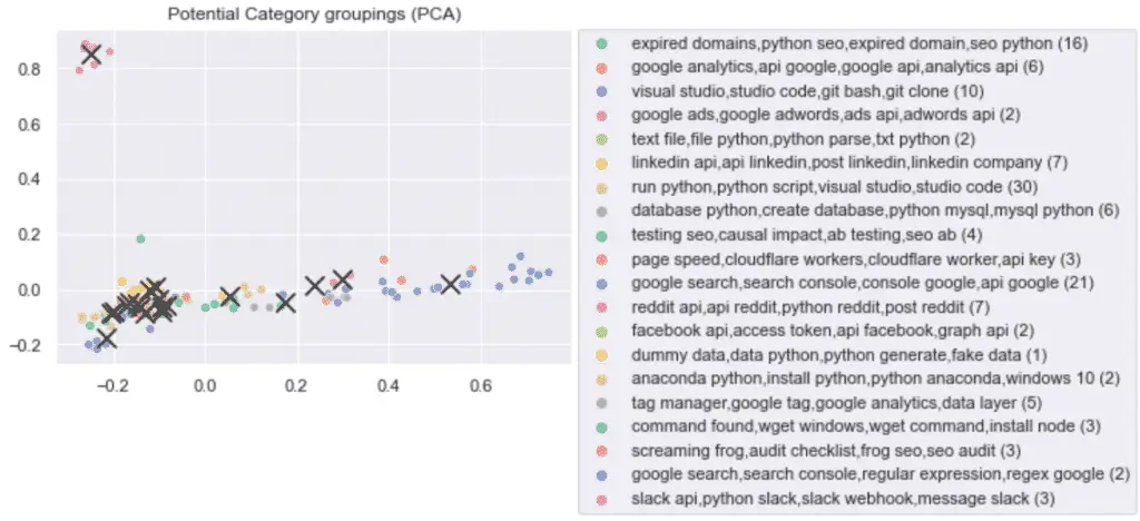
Plot the graph
Then, using Seaborn and Matplotlib, we will plot the TF-IDF PCA plot, show the KMeans cluster centroids and add a legend showing the top bigrams of each cluster.
import matplotlib.pyplot as plt
import seaborn as sns


# Plot the individual groupings
# of articles
sns.scatterplot(
    x=reduced_features[:,0],
    y=reduced_features[:,1],
    hue=labels,
    palette='Set2')

# plot the cluster centroids
plt.scatter(
    reduced_centroids[:, 0],
    reduced_centroids[:,1],
    marker='x',
    s=150,
    c='k'
    )

# plot the graph
plt.legend(bbox_to_anchor=(1.01, 1),
           borderaxespad=0)

plt.title('Potential Category groupings (PCA)')
plt.show()
Voilà!
Use the Clustered Data
We can now make the data actionable by exporting the clustered dataframe to a csv or simply printing the results to the console.
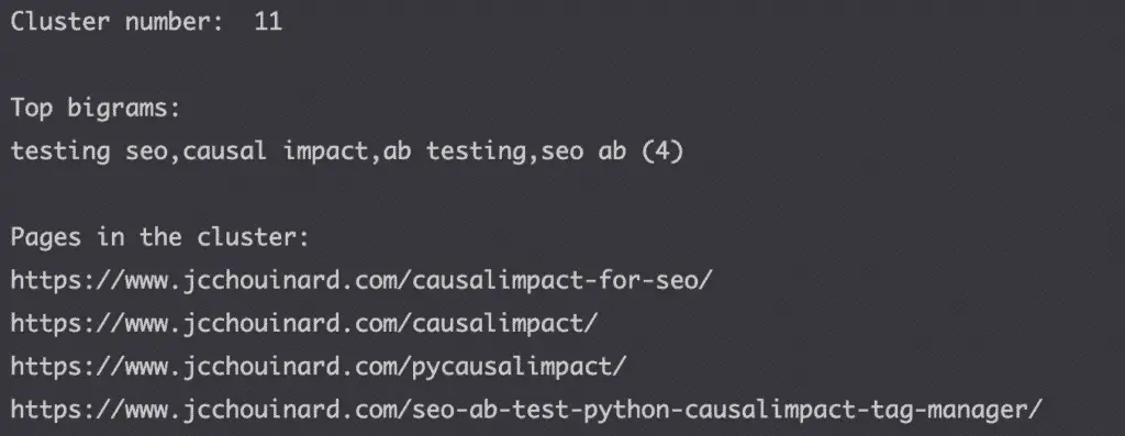
show_k = 11

print('Cluster number: ', show_k)
print('\nTop bigrams: ')
print(my_dict[show_k])
print('\nPages in the cluster: ')
pages = clusters['page'][clusters['cluster'] == show_k]
for page in pages:
    print(page)
Part 2. Identify Duplicated Pages with KMeans
Finding duplicated pages using KMeans clustering an TF-IDF is not the most effective method, but can still provide insights.
How to Identify duplicated pages using clusters?
The idea goes like this:
- Select a number of clusters that is very close to the total number of pages
- Identify the ones that get clustered together as potential duplicates.
Example:
If we create 100 clusters on 100 pages, each cluster will have 1 page.
If we create 98 clusters on 100 pages, at least 3 pages will be in cluster that has more than one page.
Thus, each cluster raises potential duplication issues.
Elbow Method: Find the Optimal number of clusters
Below, we will try to find an optimal number of clusters using the Elbow Method.
import matplotlib.pyplot as plt
import seaborn as sns

from sklearn.cluster import KMeans
from sklearn.metrics import adjusted_rand_score
sns.set()

# Run elbows in groups of 10
# Limit to a max of the total num articles
ks = [i * 10 if i*10 < len(grouped_df) else len(grouped_df) for i in range(1,15)]
sse = []

for k in ks:
    model =  KMeans(
        n_clusters=k,
        init='k-means++',
        max_iter=100,
        n_init=1)

    model.fit(X)

    sse.append(model.inertia_)

# Plot ks vs SSE
plt.plot(ks, sse, '-o')
plt.xlabel('number of clusters, k')
plt.ylabel('Sum of Squares Errors (SSE)')
plt.title('Elbow method for optimal K')
plt.axvline(x=120,linestyle='--',c='grey')
plt.axvline(x=133,linestyle='--',c='grey')
plt.xticks(ks)
plt.show()
With the elbow method, the optimal K is located where the SSE stabilizes.
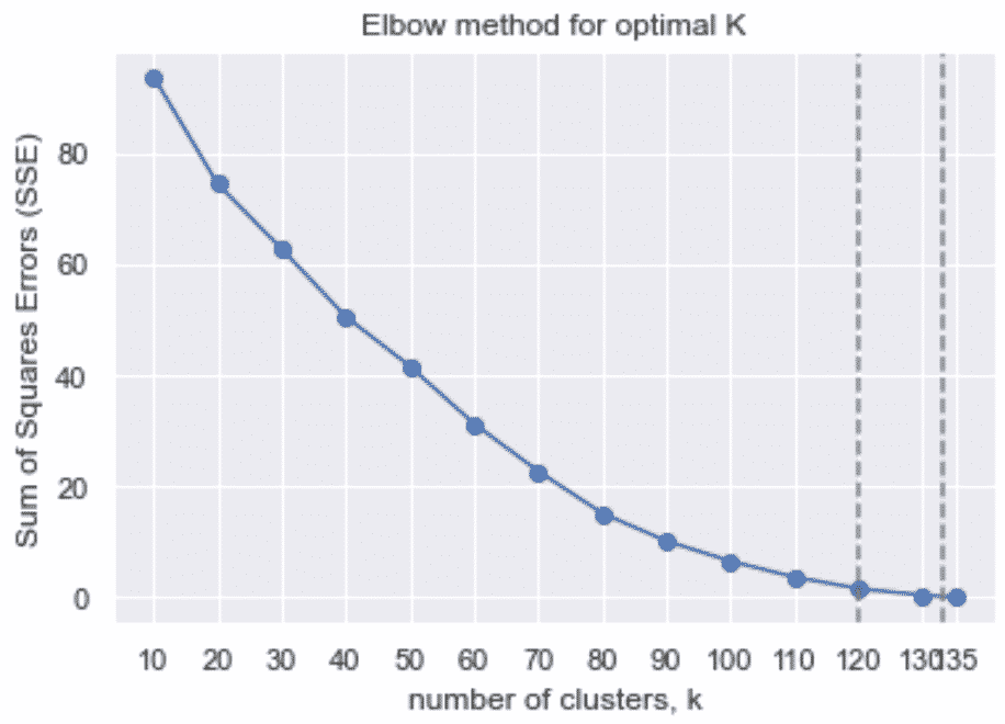
Above, we can see no clear elbow point, but the curve starts to reach stability around 120 pages out of 135.
If we cluster at 120, we may find pages that are similar, but not real duplicates. This has the risk of being too restrictive for good SEO.
But, if we cluster at 130 or above, it looks like we may manage to find true duplicated pages that may harm SEO performance.
Create a dataframe showing clustered pages
Let’s first try to group pages into 120 clusters.
from sklearn.feature_extraction.text import TfidfVectorizer
from sklearn.cluster import KMeans
from sklearn.metrics import adjusted_rand_score

# define number of clusters
k = 120

# prepare the model
model = KMeans(
    n_clusters=k,
    init='k-means++',
    max_iter=100,
    n_init=1)

# train the model
model.fit(X)

# create clustered dataframe
labels = model.labels_
mapping = list(zip(labels, grouped_df.index, queries))
clusters = pd.DataFrame(mapping, columns=['cluster','page','queries'])

# Show cluster with the most pages
lst = list(clusters['cluster'])
largest_cluster = max(lst,key=lst.count)
clusters[clusters['cluster'] == largest_cluster]
The resulting dataframe shows me the cluster with the highest number of pages.
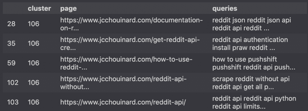
I can already see that most of these pages are about the same topic, but they do not target the same user intent.
Using 120 clusters (k=120) is too restrictive for de-duplication.
I will try using 133 K clusters.
from sklearn.feature_extraction.text import TfidfVectorizer
from sklearn.cluster import KMeans
from sklearn.metrics import adjusted_rand_score

# define number of clusters
k = 133

# prepare the model
model = KMeans(
    n_clusters=k,
    init='k-means++',
    max_iter=100,
    n_init=1)

# train the model
model.fit(X)

# create clustered dataframe
labels = model.labels_
mapping = list(zip(labels, grouped_df.index, queries))
clusters = pd.DataFrame(mapping, columns=['cluster','page','queries'])

# filter custers with more than 1 page
clusters.groupby('cluster')\
    .filter(lambda x: len(x) > 1)\
        .sort_values(by='cluster')
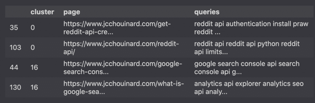
Now we are talking!
Inspecting these articles, I definitely see a possibility to either combine them or diffierentiate them better.
For example, the articles “What is search console API?” and “Google Search Console API” are both targetting a similar user’s search intent. A lot of the users that are searching for the query “Google Search Console API” want to know what it is.
Also, both articles provide the answer to that question.
They are both useful, so I can’t just merge them. I have to clarify better what each one is above.
I could potentially rename the former article to something that distinguishes its intent better, remove similar blocks of content and link to the latter using the anchor text “What is search console API?”.
Special mentions to fantastic resources on KMeans
Congratulations for making it this far. I couldn’t have written this post without the help of fantastic people in the community. Have a look at these articles to learn more about how to use KMeans.
- NLP with Python: Text Clustering by Sanjaya Subedi
- K-Means Clustering with scikit-learn by Jonathan Soma
- SEO – Kmeans clustering by Konrad Burchardt
- Python for SEO using Google Search Console by Shrikar Archak
- Kmeans text clustering
- Clustering documents with Python by Dimitris Panagopoulos on towardsdatascience
- Comparing the performance of non-supervised vs supervised learning methods for text classification
- K-Means Clustering – The Math of Intelligence – by Siraj Raval
Conclusion
That was a lot. We have learned how to create clusters based on Google Search Console queries using KMeans, TF-IDF and PCA.

SEO Strategist at Tripadvisor, ex- Seek (Melbourne, Australia). Specialized in technical SEO. Writer in Python, Information Retrieval, SEO and machine learning. Guest author at SearchEngineJournal, SearchEngineLand and OnCrawl.