Principal Component Analysis is a technique that simplifies complex data by finding and keeping only the most important patterns or features.
What is Principal Component Analysis (PCA)?
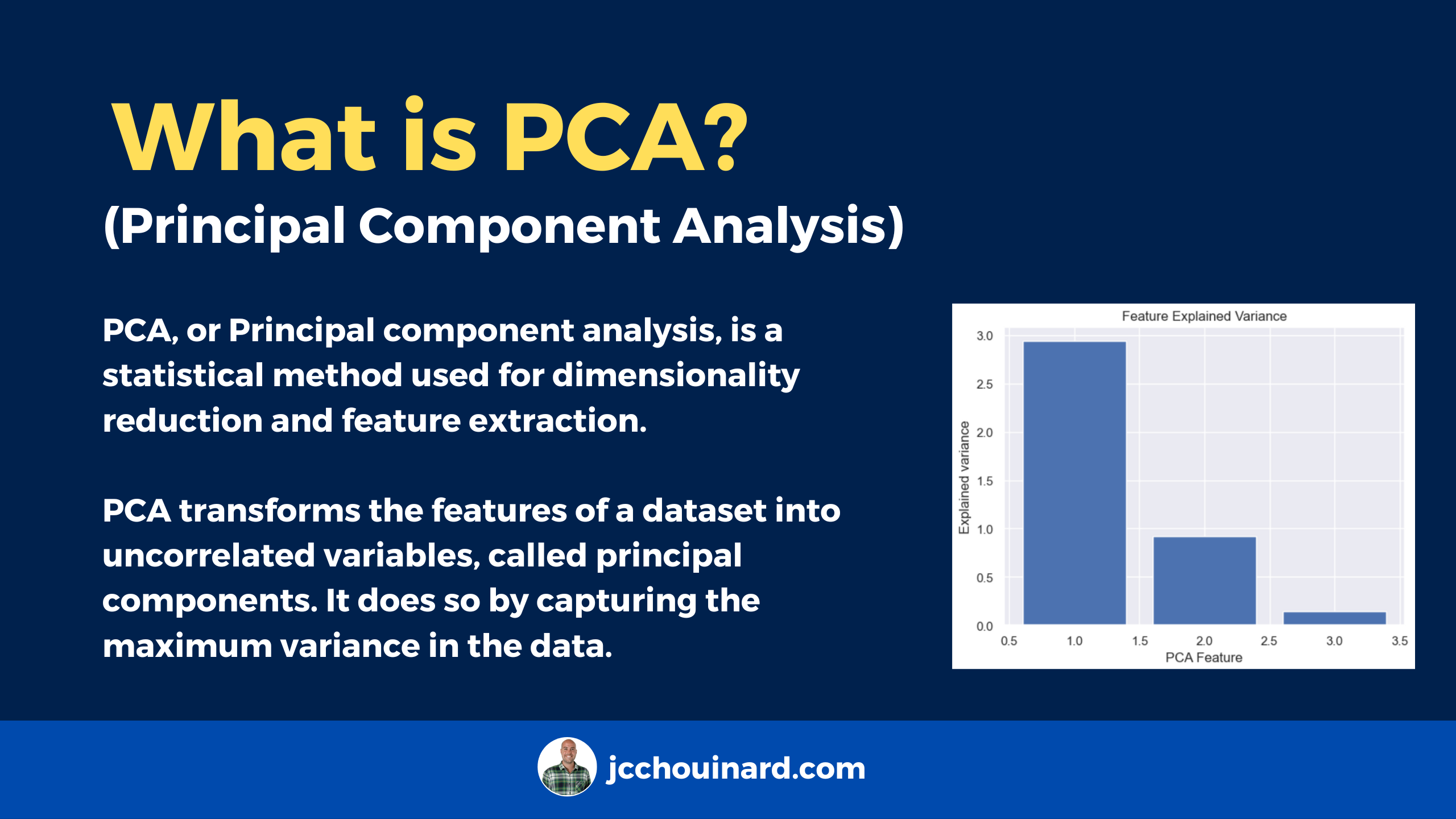
Principal Component Analysis (PCA) is a linear dimensionality reduction technique used to extract information from high-dimensional datasets. PCA performs dimension reduction by projecting data into a lower-dimensional space, trying to preserve components with higher variation while discarding those with lower variation.
In simple words, PCA tries to reduce the number of dimension to its principal components whilst retaining as much variation in the data as possible. PCA is the main linear algorithm for dimension reduction often used in unsupervised learning.
Principal Component Analysis was first introduced by Karl Pearson in 1901 on a paper titled “On lines and planes of closest fit to systems of points in space”.
PCA transforms the features of a dataset into uncorrelated variables, called principal components. It does so by capturing the maximum variance in the data. Dimension reduction is generally used to overcome the curse of dimensionality.
What are Principal Components in PCA?
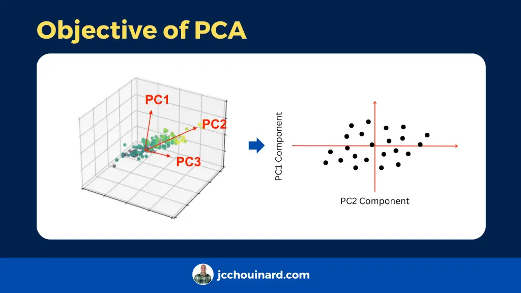
Principal components (PC) in PCA are a specific linear combination that are used to reduce large dimensional datasets to data sets with fewer dimensions, while keeping most of the information in the original data matrix. Principal components are chosen in a way that each one have the following characteristics:
- Principal components are uncorrelated
- Ordered so that the first principal component explains the largest percentage of variation in the original dataset, the second explains the second largest percentage, and so on.
According to the original DATAPLOT reference manual, principal components allow to simplify many data analyses, but has the disadvantage of making the interpretation more difficult by affecting the scaling and loosing the original variables.
Dimensions represent features in the data.
This algorithm identifies and discards features that are less useful to make a valid approximation on a dataset.
Why use PCA?
Python and PCA help reducing the number of features in a dataset and can help:
- Reduce the risk of overfitting a model to noisy features.
- Speed-up the training of a machine learning algorithm
- Make simpler data visualizations.
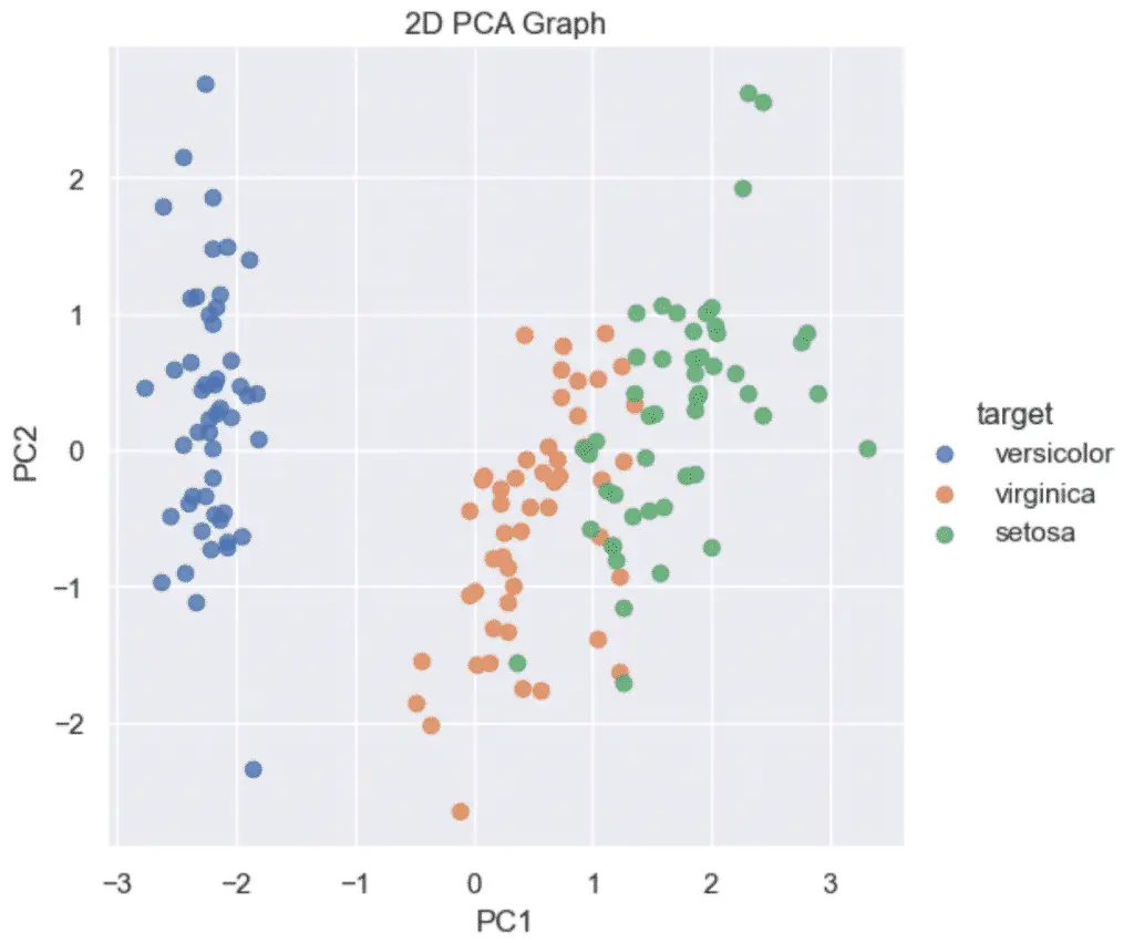
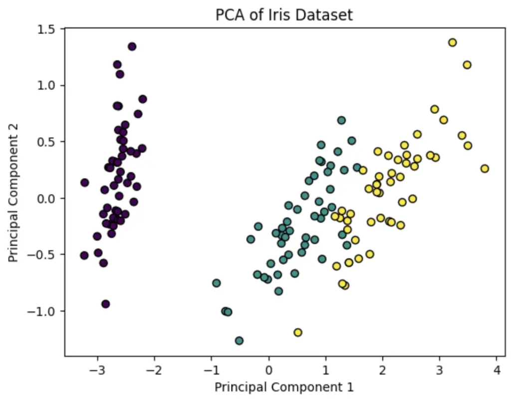
Let’s make an example with the Iris dataset. The dataset has 4 features: sepal and petal length and width… hard to plot a 4D graph.
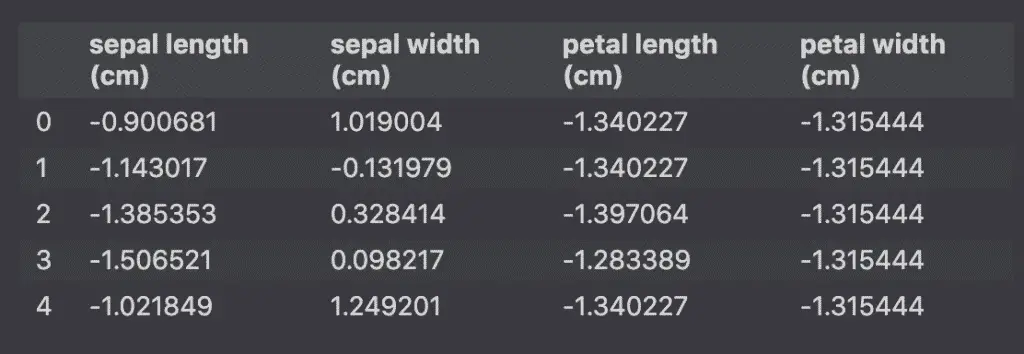
However, we can use PCA to reduce the number of features to plot the data on a 2D graph. (se how to plot PCA).
Interestingly, it can do cool things like remove background from an image.

Advantages and Disadvantages of PCA
| PCA Advantages | PCA Disadvantages |
|---|---|
| Reduce Noise in the Data | Risk loss information |
| Improve Visualization With Less Dimension | Not meant for non-linear datasets. Use non-linear dimensionality reduction techniques instead |
| Improve Training Efficiency | Expensive run-time on large dataset |
| Reduce Machine Learning Parameters | Impacted by outliers |
Principal Component Analysis Generalizations
To fix some to the disadvantages of PCA, alternative principal component analysis techniques were created.
- Sparse Principal Component Analysis
- Kernel Principal Component Analysis
What is Sparse Principal Component Analysis
Sparse principal component analysis (SPCA or sparse PCA) is a specialised technique used in statistical analysis and, in particular, in the analysis of multivariate data sets. According to a paper published in the Journal of Computational and Graphical Statistics by Hui Zou and al, sparse PCA improves data processing and dimensionality reduction by using the lasso (elastic net) to produce modified principal components with sparse loadings. [1]
What is Kernel Principal Component Analysis
Lernel principal component analysis (KPCA) is nonlinear generalization that acts as an extension of principal component analysis using techniques of kernel methods (Kernel trick). The standard KPCA algorithm was introduced in the field of multivariate statistics by Schölkopf et al in “Nonlinear Component Analysis as a Kernel Eigenvalue Problem” (1998), proving to be a powerful approach to extracting nonlinear features in classification and regression problems, but may be computationally expensive in larger scale datasets.
What is Robust Principal Component Analysis
Robust Principal Component Analysis is a modification of the widely used statistical procedure of principal component analysis which works well with respect to grossly corrupted observations.
What is Functional Principal Component Analysis
Functional principal component analysis is a statistical method for investigating the dominant modes of variation of functional data.
What is L1-norm principal component analysis
L1-norm principal component analysis is a general method for multivariate data analysis. L1-PCA is often preferred over standard L2-norm principal component analysis when the analyzed data may contain outliers.
What is Multilinear principal component analysis
Multilinear principal component analysis is a multilinear extension of principal component analysis. MPCA is employed in the analysis of M-way arrays, i.e. a cube or hyper-cube of numbers, also informally referred to as a “data tensor”.
What is Principal Component Regression
Principal component regression is a regression analysis technique based on principal component analysis. More specifically, PCR is used for estimating the unknown regression coefficients in a standard linear regression model.
Introduction to PCA in Python
Here is a simple example of Principal Component Analysis in Python where we perform dimension reduction on the Iris dataset with Scikit-learn.
import matplotlib.pyplot as plt
from sklearn.decomposition import PCA
from sklearn.datasets import load_iris

# Load Iris dataset (for illustration purposes)
iris = load_iris()
X = iris.data
y = iris.target

# Apply PCA with two components (for 2D visualization)
pca = PCA(n_components=2)
X_pca = pca.fit_transform(X)

# Plot the results
plt.scatter(X_pca[:, 0], X_pca[:, 1], c=y, cmap='viridis', edgecolor='k')
plt.title('PCA of Iris Dataset')
plt.xlabel('Principal Component 1')
plt.ylabel('Principal Component 2')
plt.show()
Read our in-depth tutorial showing PCA Python Examples.

SEO Strategist at Tripadvisor, ex- Seek (Melbourne, Australia). Specialized in technical SEO. Writer in Python, Information Retrieval, SEO and machine learning. Guest author at SearchEngineJournal, SearchEngineLand and OnCrawl.