What are PCA Loadings (with Python Example)

In Principal Component Analysis (PCA), loadings represent the contribution of each original variable to the principal component. PCA loadings are used to understand patterns and relationships between variables. They help identify which variables contribute most to each of the Principal Components.

While PCA reduces the dimensionality of a dataset, loadings are the coefficients assigned to each original variable that is used to create the principal component.

When to Use PCA Loadings

PCA loadings are often used in loading plots and biplots to evaluate the importance PCA Features.

Python Example of PCA Loadings

Here, we will apply PCA with Python and then produce a Pandas Dataframe containing the PCA loadings:

import numpy as np
import pandas as pd
import matplotlib.pyplot as plt
from sklearn.decomposition import PCA
from sklearn.datasets import load_iris
from sklearn.preprocessing import StandardScaler

# Load Iris dataset 
iris = load_iris()
X = iris.data
y = iris.target

# Standardize the data
scaler = StandardScaler()
X_standardized = scaler.fit_transform(X)

# Apply PCA with two components 
pca = PCA(n_components=2)
X_pca = pca.fit_transform(X_standardized)

# Extract loadings
loadings = pca.components_.T * np.sqrt(pca.explained_variance_)

# Create a DataFrame for loadings
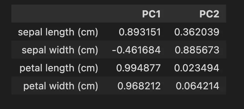
loadings_df = pd.DataFrame(loadings, columns=['PC1', 'PC2'], index=iris.feature_names)
loadings_df

How to Interpret PCA Loadings

In PCA, loadings indicate the contribution of each original feature to the principal components.

• Positive or negative: direction of the relationship.
• Higher absolute values: stronger contribution to principal components.

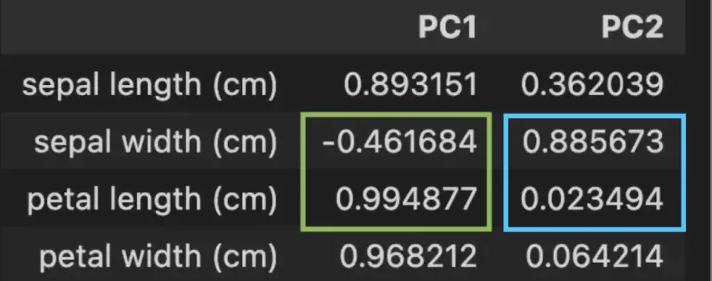
In the loading Dataframe above, we can see that the petal length is the most important contributor to the variability of the Principal Component 1 with a coefficient of 99.5%. An increase in petal length corresponds to a higher value of PC1. We can also see that sepal width contributes negatively. Meaning that an increase in sepal width corresponds to a lower value of PC1.

In Blue, we see that sepal width is the strongest contributor and petal length the weakest to the PC2.

Difference Between Loadings, Correlation Coefficients and Eigenvectors

PCA loadings, correlation coefficients and eigenvectors are related but not exactly the same.

• explained variance: Amount of variance explained by each principal component. pca.explained_variance_
• eigenvectors: direction of maximum variance, unit-scaled loadings: pca.components_
• loadings: contribution of variables to the principal components. eigenvectors * sqrt(explained variance)
• correlation coefficients: strength and direction of linear relationship between two variables. np.corrcoef()

Loadings are influenced by correlations, but also consider the variability of each variables. Eigenvectors and loadings are simply two different ways to normalize the data points. Loadings and correlation coefficients are complementary in analyzing relationships.

import numpy as np
import pandas as pd
import matplotlib.pyplot as plt
from sklearn.decomposition import PCA
from sklearn.datasets import load_iris
from sklearn.preprocessing import StandardScaler

# Load Iris dataset
iris = load_iris()
X = iris.data
y = iris.target

# Standardize the data
scaler = StandardScaler()
X_standardized = scaler.fit_transform(X)

# Apply PCA with two components
pca = PCA(n_components=2)
X_pca = pca.fit_transform(X_standardized)

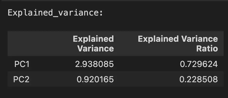
explained_variance = pca.explained_variance_
print("Explained_variance:")
pd.DataFrame({
    'Explained Variance': explained_variance,
    'Explained Variance Ratio': pca.explained_variance_ratio_,
}, index=['PC1', 'PC2'])

The explained variance shows that the PC1 contributes the most to the variance in the data.

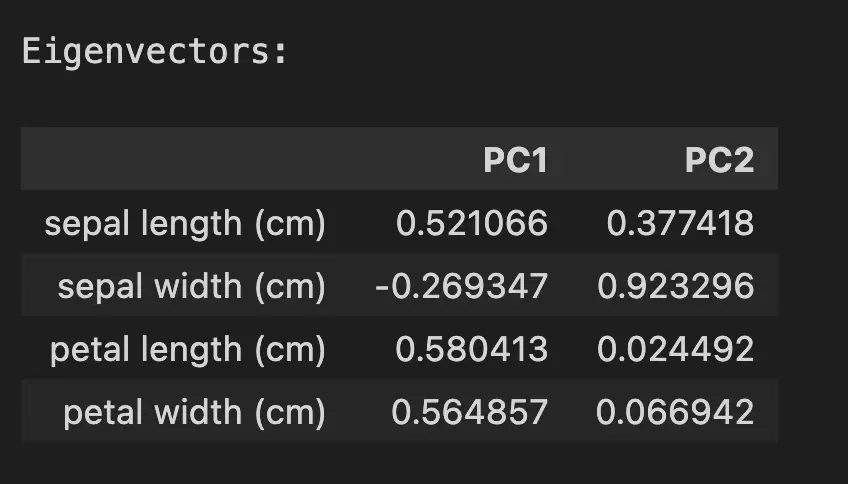
print("\nEigenvectors:")
eigenvectors = pca.components_
pd.DataFrame(eigenvectors, columns=iris.feature_names, index=['PC1', 'PC2']).T

The eigenvectors shows the main direction of the maximum variance, using the same unit-scale as the explained variance. In the context of PCA, eigenvectors are often referred to as modes of variation. For example, sepal width seem to impact PC1 and PC2 in different directions.

print("\nLoadings:")
loadings = eigenvectors.T * np.sqrt(explained_variance)
pd.DataFrame(loadings, columns=['PC1', 'PC2'], index=iris.feature_names)

The loadings are scaled versions of the eigenvector * square root of the explained variance so that it shows, not only the direction (like with eigenvectors), but also the magnitude of the variance.

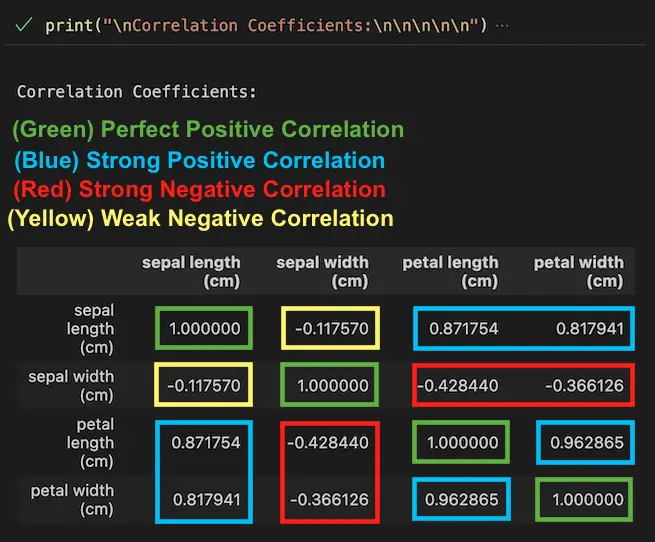
print("\nCorrelation Coefficients:")
correlation_coefficients = np.corrcoef(X_standardized, rowvar=False)
pd.DataFrame(correlation_coefficients, columns=iris.feature_names, index=iris.feature_names)

The correlation coefficients show the correlation between variables.

1. Perfect Positive Correlation (1.0)
2. Strong Positive Correlation (Close to 1.0)
3. Strong Negative Correlation (Close to -1.0)
4. Weak Correlation (Close to 0)

In summary, PCA loadings and correlation coefficients are important in understanding the relationships and patterns in multivariate data. While they have different interpretations, they complement each other in providing insights into the underlying structure of the data.

Jean-Christophe Chouinard

SEO Strategist at Tripadvisor, ex- Seek (Melbourne, Australia). Specialized in technical SEO. Writer in Python, Information Retrieval, SEO and machine learning. Guest author at SearchEngineJournal, SearchEngineLand and OnCrawl.