The curse of dimensionality refers the the various challenges of making meaningful machine learning generalizations from data containing large number of dimensions.
What is the Curse of Dimensionality?
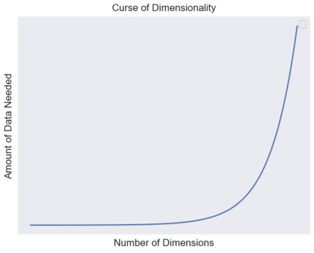
The Curse of Dimensionality explains how as the number of dimension or features increases, the amount of data we need to make accurate generalizations grows exponentially.
The term was coined by Richard E. Bellman in 1966 in a paper name Dynamic programming refers to the challenges that arise when working with data in high-dimensionality. Objects tend to become more sparse and dissimilar, making it harder to gather meaningful insights from the data.
Curse of Dimensionality Example
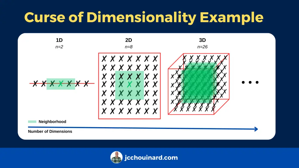
An example of the curse of dimensionality is when we try to find the k-nearest neighbours of a value. When you have a 1 dimensional line, and all the data spread uniformly across that line, the nearest neighbour will default to a very small neighbourhood of possible values.
- 1D: each X represents 1/6th, n_neighbors=2, distance is small
- 2D: each X represents 1/36th, n_neighbors=8, distance is medium
- 3D: each X represents 1/216th, n_neighbors=26, distance is large
- …
Why the Curse of Dimensionality Matters?
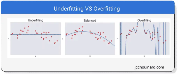
The curse of dimensionality matters because large number of dimensions tend to lead to underfitting or overfitting.
Models are influenced by Distance
A lot of machine learning models (such as KNN, K-Means and Decision Trees) are heavily influenced by the distances between data points. By adding more data points, the relative distance increase exponentially. The more dimensions, the fewer data points per dimension that you have.
When Does Overfitting Occurs?
Overfitting occurs when the model memorizes all training examples and doesn’t generalize well to unseen data. To avoid overfitting, the number of observations should increase exponentially with the number of features.
If you have all this additional information, but do not increase the number of data points, the model will have a hard time making sense of unseen data. This is when the curse of dimensionality leads to overfitting de data.
You can evaluate overfitting by looking at the accuracy_score on the training data vs the accuracy_score on the testing data. Here is a non-scientific rule-of-thumb to estimate overfitting based on the difference between training and test set accuracy.
No Overfitting: difference less than 2-3%.Mild Overfitting: difference between 3-5%Significant Overfitting: difference between 5-10%Strong Overfitting: difference greater than 10%
Here is a simple example of low overfitting.
from sklearn.datasets import load_wine
from sklearn.model_selection import train_test_split
from sklearn.tree import DecisionTreeClassifier
from sklearn.metrics import accuracy_score

# Load the wine dataset
data = load_wine()
X, y = data.data, data.target

# Split the data into training and test sets
X_train, X_test, y_train, y_test = train_test_split(X, y, test_size=0.3, random_state=42)

# Train a DecisionTreeClassifier
clf = DecisionTreeClassifier(random_state=42)
clf.fit(X_train, y_train)

# Calculate accuracy on the training and test sets
accuracy_train = accuracy_score(y_train, clf.predict(X_train))
accuracy_test = accuracy_score(y_test, clf.predict(X_test))

print(f"Training set accuracy: {accuracy_train:.1%}")
print(f"Test set accuracy: {accuracy_test:.1%}")
print(f"Difference: {accuracy_train - accuracy_test:.1%}")
Training set accuracy: 100.0%
Test set accuracy: 96.3%
Difference: 3.7%
When Does Underfitting Occurs?
When you add too many dimensions (e.g. time of the day, ice cream brand, etc.), the model has a hard time to make sense of all that noise. The curse of dimensionality leads to underfitting the data.
This often happens when you want to make simple predictions (e.g. ice cream sales and temperature).
Example with Mild underfitting
from sklearn.datasets import load_iris
from sklearn.model_selection import train_test_split
from sklearn.svm import SVC
from sklearn.metrics import accuracy_score

# Load the Iris dataset
iris = load_iris()
X, y = iris.data, iris.target

# Split into training and test sets
X_train, X_test, y_train, y_test = train_test_split(X, y, test_size=0.3, random_state=42)

# Create SVC model and train it
svc = SVC()
svc.fit(X_train, y_train)


accuracy_train = accuracy_score(y_train, svc.predict(X_train))
accuracy_test = accuracy_score(y_test, svc.predict(X_test))

print(f"test set accuracy: {accuracy_test:.1%}.")
print(f"Training set accuracy: {accuracy_train:.1%}")
print(f'Difference: {(accuracy_train - accuracy_test):.1%}')
test set accuracy: 100.0%.
Training set accuracy: 96.2%
Difference: -3.8%
Finding the True Dimensionality of a Dataset
This works because datasets are generally high-dimensional because we choose to make them high dimensional.
When we have documents, we choose to perform things such as TF-IDF to make each word become its own attribute, further increasing the number of dimensions.
The dataset’s true dimensionality is generally much lower.
How to Overcome the Curse of Dimensionality?
There are three main ways to overcome the curse of dimensionality: dimensionality reduction, increase in the number of data points and feature engineering.
Dimensionality Reduction
You can perform dimension reduction using tools like principal component analysis on a dataset. This will reduce the number of features by selecting only the principal components that contribute the most to the variance in the data.
Increase in Data Points
Adding more data points (not features) to the dataset will make the models less subject to variations from the input training data.
Feature Engineering
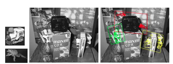
By using domain knowledge to extract features from the dataset (feature engineering). For example, you could use the SIFT algorithm to select a part of an image and train the data only on the dimensions related to that part.
Other techniques to reduce high dimensionality can be:
- Derivation: Evaluate each dimension independently
- Smoothing: Spread class to neighbors
- Symmetry: Reduce number of configurations of the same pattern

SEO Strategist at Tripadvisor, ex- Seek (Melbourne, Australia). Specialized in technical SEO. Writer in Python, Information Retrieval, SEO and machine learning. Guest author at SearchEngineJournal, SearchEngineLand and OnCrawl.