In this tutorial, you will learn how to identify the importance of the original features in the reduced dataset. If we had 5 features and reduced to 3, which ones were the most important?
We assume that you have identified the reduced Principal Components (PC) that explained most of the variance in the dataset. Now, we want to know which feature are important in the remaining Principal Components after dimension reduction.
How to Identify PCA Feature Importance in Python
To identify the contribution of original features to each principal component (PC), use the explained variance ratio for each component using explained_variance_ratio_ attribute on the pca object.
This example applies Principal Component Analysis on the Iris dataset, using Scikit-learn.
import matplotlib.pyplot as plt
from sklearn.decomposition import PCA
from sklearn.datasets import load_iris

# Load Iris dataset
iris = load_iris()
X = iris.data
y = iris.target

# Apply PCA with two components
pca = PCA(n_components=2)
X_pca = pca.fit_transform(X)

# Explained Variance Ratio
pca.explained_variance_ratio_
The higher the explained variance ratio, the more important the principal component is in explaining the variance of the data.
array([0.92461872, 0.05306648])Here, we have an array where 92% of the variance is explained by the first principal component (PC1) and the 5% is explained by PC2. Together, they explain 97% of the variance of the data.
To learn how PCA works in Python, see our PCA Sklearn example in Python.
How to Identify the Importance of Each Original Feature
To identify the importance of each feature on each component, use the components_ attribute.
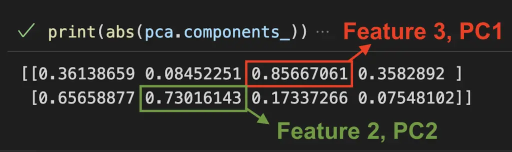
print(abs(pca.components_))
The result is an array containing the PCA loadings in which “rows” represents components and “columns” represent the original features.
[[0.36138659 0.08452251 0.85667061 0.3582892 ]
 [0.65658877 0.73016143 0.17337266 0.07548102]]
Here we can estimate that the third feature explained 86% of the first principal component and the second feature explained 73% of the second principal component.
The next steps in understanding the importance of each features is to:
What is the Explained Variance?
The explained variance, or eigenvalue, in PCA shows the variance that can be attributed to each of the principal components.
The larger the eigenvalue, the more important the corresponding eigenvector is in explaining the variance of the data.
It is an array of values where each value equals the variance of each principal component and the length of the array is equal to the number of components defined with n_components.
It can be accessed with the .explained_variance_ notation.
pca.explained_variance_
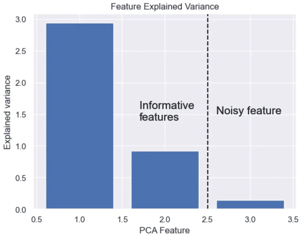
array([2.93808505, 0.9201649 ])
How to Plot the Explained Variance in Python
The explained variance in PCA helps us understand how much information is retained after dimensionality reduction. It is the portion of the original data’s variability that is captured by each principal component.
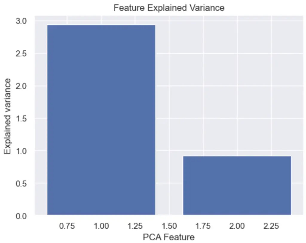
We can plot the explained variance to see the variance of each principal component feature.
# Bar plot of explained_variance
plt.bar(
    range(1,len(pca.explained_variance_)+1),
    pca.explained_variance_
    )

plt.xlabel('PCA Feature')
plt.ylabel('Explained variance')
plt.title('Feature Explained Variance')
plt.show()
The output graph shows that 1 of the PCA features is obviously more significant than the other.
Read our tutorial on the best PCA plots in Python for more data visualization examples with PCA and Python.

SEO Strategist at Tripadvisor, ex- Seek (Melbourne, Australia). Specialized in technical SEO. Writer in Python, Information Retrieval, SEO and machine learning. Guest author at SearchEngineJournal, SearchEngineLand and OnCrawl.