This is the last part of our guide on how to set up your own SEO split tests with Python, R, the CausalImpact package and Google Tag Manager.
Step 1: Install Python and R Using Anaconda
Step 2: Stratified Sampling Using Google Analytics + Python
Step 3: SEO Split-Testing Experiments using Google Tag Manager
Step 4: CausalImpact for SEO [Complete DIY SEO Experiment]
(Optional) Learn python for SEO
We will use R and the CausalImpact package to compare our test results to what we should have expected. Follow this article If you would wish to run CausalImpact in Python.
How CausalImpact Works?
There are plenty of resources that explain how CausalImpact works, but just watch the video to understand the underlying principle.
Basically, in an SEO split-testing experiment, the package uses Bayesian statistics to predict what should be your traffic if you do nothing.
Then, it compares what you should have expected (predicted from the control group) to what really happened (your test group).
Getting Started
To run CausalImpact you will need a few things to get started.
Step 1: Install Packages and Load Libraries
To run CausalImpact on Google Analytics data, we will need to install RGoogleAnalytics and googleAuthR packages.
##### Step 1: Install packages and load libraries ####

Packages      <- c("RGoogleAnalytics","googleAuthR","xlsx","CausalImpact","bsts")

# Look if packages are installed, if not, install them.
new.packages  <- Packages[!(Packages %in% installed.packages()[,"Package"])]
if(length(new.packages)) install.packages(new.packages)

# Load all libraries
lapply(Packages, library, character.only = TRUE)
Step 2: Authenticate to the API
To use the Google Analytics API, we need to connect to it. You will need your client.id and client.secret. To get it, read how to connect to a Google API.
## Add your own client.id and client.secret.

client.id         <- "XXXXXXXXXXXXXXXXXXX.apps.googleusercontent.com"
client.secret     <- "XXXXXXXXXXXXXXXXXXX"
token             <- Auth(client.id,client.secret)
Here, a pop-up will open in your browser asking you to authenticate.

Great.
Save the authentication token so you don’t need to authorize each time.
#### Save authentication token ####

save(token,file="./token_file")
ValidateToken(token)
Step 3: Setup Your Extractor Variables
In this part, you will write down what you want to track. Add your own website, your own UA tracking code and set your intervention dates.
website          <- "https://www.example.com"         # Add your own website
UA               <- "ga:XXXXXXXXXX"                   # Add your own View ID
startDate        <- as.Date("2019-01-01")
endDate          <- as.Date("2020-01-01")
InterventionDate <- as.Date("2019-10-01")
time.points      <- as.Date(seq(startDate,endDate,by="day"))
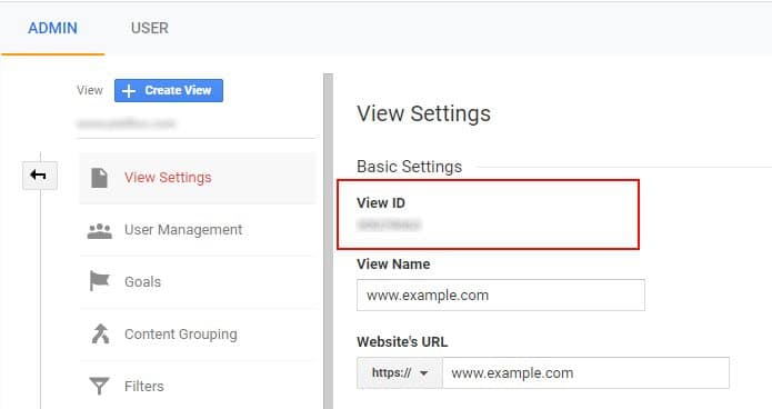
You will find your profile ID in Google Analytics > Admin > View > View Settings > View ID. This is your “UA” variable.
The interventiondate is the moment when you change occurred. The time.points variable is used to convert dates as a time series.
Step 4: Set the Intervention
The intervention is the dataset on which you have tested something.
The testpages variable is the set of pages that you have gathered in the post on stratified sampling. You can add any URL you want by specifying the page path in the Regex.
If you don’t know much about Regex, read my guide on Regular expressions.
The gaFilters variable can stay as it is. It currently extracts Google’s organic traffic for your test pages. You can set your own using Query Explorer.
testPages  <- "^/test-page-1.*|^/test-page-2.*|^/test-page-3.*|^/test-page-n.*"  # Add your own test pages
gaFilters  <- paste("ga:sourceMedium==google / organic;ga:landingPagePath=~",testPages,sep="")
The code below makes the API call for you, selecting the startDate, endDate and filters that you specified and extracting the sessions by day.
query.list <-Init(start.date = as.character(startDate),
                  end.date = as.character(endDate),
                  dimensions = "ga:date",
                  filters = gaFilters,
                  metrics = "ga:sessions",
                  max.results = 50000,
                  sort = "ga:date",
                  table.id = UA)

ga.query  <- QueryBuilder(query.list)
ga.data   <- GetReportData(ga.query,token,split_daywise = T)
test      <- ga.data
Step 5: Set Predictor Variable
The predictor variable, also known as the control group, will help you compare the tested data to other pages that haven’t had the change.
This step is similar to what we did before. We will only log the result into the control variable instead of the test variable.
You have two options available here: test your data against a control group (large sites), test your data against the entire website (smaller sites).
controlPages  <- "^/control-page-1.*|^/control-page-2.*|^/control-page-3.*|^/control-page-n.*"  # Add your own control pages

## Option 1 : Compare to a control group
gaControlFilters1  <- paste("ga:sourceMedium==google / organic;ga:landingPagePath=~",controlPages,sep="")
## Option 2 : Compare to the entire site
# gaControlFilters2  <- paste("ga:sourceMedium==google / organic;ga:landingPagePath!~",testPages,sep="")

query.list <-Init(start.date = as.character(startDate),
                  end.date = as.character(endDate),
                  dimensions = "ga:date",
                  filters = gaControlFilters1,
                  #filters = gaControlFilters2,
                  metrics = "ga:sessions",
                  max.results = 50000,
                  sort = "ga:date",
                  table.id = UA)

ga.query   <- QueryBuilder(query.list)
ga.data    <- GetReportData(ga.query,token,split_daywise = T)
control    <- ga.data
Step 6: Convert Variables to a Time Series
Next, we want to work with time series. This is why we are going to convert Intervention and predictor as a time series using ts.
test       <- ts(test[2])
control    <- ts(control[2])
Step 7: Plot Causal Impact
Now it is time to plot our data.
Convert Dates Into Vectors
The first part of the code below converts date to numbers. This way I can create a usable vector for the formula. You have nothing to change.
## Find Date as Number to create a usable vector (Intervention - start = Number of days between dates)
InterventionDateNum   <- as.Date(strptime(as.character(InterventionDate), "%Y-%m-%d"))-as.Date(strptime(as.character(startDate), "%Y-%m-%d"))
InterventionDateNum   <- as.numeric(InterventionDateNum)
totalDateNum          <- as.Date(strptime(as.character(endDate), "%Y-%m-%d"))-as.Date(strptime(as.character(startDate), "%Y-%m-%d"))+1
totalDateNum          <- as.numeric(totalDateNum)
Set Pre and Post Period
Add the pre and post period of your experiment using the Intervention date as a delimiter.
## Set Pre and Post Period
pre.period            <- c(1,InterventionDateNum)
post.period           <- c(InterventionDateNum,totalDateNum)
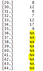
Remove Post Period Data to be Replaced by Prediction
Now, we remove the data after the intervention in the test group.
## Remove Data from Post Period
post.period.response <- test[post.period[1] : post.period[2]]
test[post.period[1] : post.period[2]] <- NA
CausalImpact will repopulate this data with the predicted data from the control group to make the comparison.
It is now time to compute the BSTS model.
Compute BSTS Model
I decided to use a custom model using BSTS because it is more precise. It lets me add a weekly (season.duration=7) and a yearly seasonal trend (nseasons=52).
## Compute BSTS Model
ss <- AddLocalLevel(list(), test)
ss <- AddSeasonal(ss,y,nseasons=52,season.duration=7) # https://rdrr.io/cran/bsts/man/bsts.html
bsts.model <- bsts(test ~ control, ss, niter = 1000)  # intervention depends on predictor
The local level model assumes the trend is a random walk. Normal distribution.
The ss=state.specification is just a list with a particular format.
The AddLocalLevel adds a random distribution to an empty state specification (the list() in its first argument). Learn more.
AddSeasonal adds a seasonal state component (nseasons) with 52 seasons (or 52 weeks) to the state specification created on the previous line.
The seasonal.duration component is telling how long each season should last (7 days). A little trick to add 2 seasonal components to the bsts model.
Plot the data
## Plot CausalImpact
impact <- CausalImpact(bsts.model = bsts.model,post.period.response = post.period.response)
plot(impact)
summary(impact)
impact$summary
summary(impact, "report")
Step 8: Analyze Data
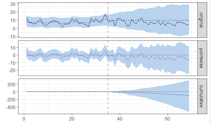
To understand the graph below you need to understand basic statistical analysis.
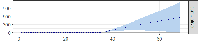
The blue shaded area represents your confidence interval (CI). You can see that the shaded area increases. Why?
Since the longer the predicted period, the less reliable the prediction is.

The test is significant when the shaded area crosses zero (or when the p-value is less than 0.05 in a 95% CI)
You can analyze your data further by using built-in CausalImpact reports.
summary(impact)
impact$summary
summary(impact, "report")
Full R Code
"Make sure your environment is clear. If you want to restart your R Session from scratch, CTRL+Shift+C to uncomment all."

#.rs.restartR()
#rm(list=ls())
#cat("\014")

##### Step 1: Install packages and load libraries ####

Packages      <- c("RGoogleAnalytics","googleAuthR","xlsx","CausalImpact","bsts")

# Look if packages are installed, if not, install them.
new.packages  <- Packages[!(Packages %in% installed.packages()[,"Package"])]
if(length(new.packages)) install.packages(new.packages)

# Load all libraries
lapply(Packages, library, character.only = TRUE)

#### Step 2: Authenticate ####

## Add your own client.id and client.secret.
## To know how https://www.jcchouinard.com/google-api/.

client.id         <- "XXXXXXXXXXXXXXXXXXX.apps.googleusercontent.com"
client.secret     <- "XXXXXXXXXXXXXXXXXXX"
token             <- Auth(client.id,client.secret)

#### Save authentication token ####

save(token,file="./token_file")
ValidateToken(token)

##### Step 3: Setup testing period #####

## Add profile ID: Google Analytics > Admin > View > View Settings > View ID
## To know how https://www.jcchouinard.com/google-api/.

website          <- "https://www.example.com"         # Add your own website
UA               <- "ga:XXXXXXXXXX"                   # Add your own View ID
startDate        <- as.Date("2019-10-09")
endDate          <- as.Date("2019-12-16")
InterventionDate <- as.Date("2019-11-14")
time.points      <- as.Date(seq(startDate,endDate,by="day"))


#### Step 4: Set Intervention #####

#### Call GA API #####
testPages  <- "^/test-page-1.*|^/test-page-2.*|^/test-page-3.*|^/test-page-n.*"  # Add your own test pages
gaFilters  <- paste("ga:sourceMedium==google / organic;ga:landingPagePath=~",testPages,sep="")

query.list <-Init(start.date = as.character(startDate),
                  end.date = as.character(endDate),
                  dimensions = "ga:date",
                  filters = gaFilters,
                  metrics = "ga:sessions",
                  max.results = 500000,
                  sort = "ga:date",
                  table.id = UA)

ga.query  <- QueryBuilder(query.list)
ga.data   <- GetReportData(ga.query,token,split_daywise = T)
test      <- ga.data #y


#### Step 5: Set Predictor #####

controlPages  <- "^/control-page-1.*|^/control-page-2.*|^/control-page-3.*|^/control-page-n.*"  # Add your own control pages

## Option 1 : Compare to a control group
gaControlFilters1  <- paste("ga:sourceMedium==google / organic;ga:landingPagePath=~",controlPages,sep="") #use ";" for "and" and "," for "or"
## Option 2 : Compare to the entire site
# gaControlFilters2  <- paste("ga:sourceMedium==google / organic;ga:landingPagePath!~",testPages,sep="")

query.list <-Init(start.date = as.character(startDate),
                  end.date = as.character(endDate),
                  dimensions = "ga:date",
                  filters = gaControlFilters1,
                  #filters = gaControlFilters2,
                  metrics = "ga:sessions",
                  max.results = 50000,
                  sort = "ga:date",
                  table.id = UA)

ga.query   <- QueryBuilder(query.list)
ga.data    <- GetReportData(ga.query,token,split_daywise = T)
control    <- ga.data


##### Step 6: Convert Intervention and predictor as a time series #####

test       <- ts(test[2])
control    <- ts(control[2])


##### Step 7: Plot BSTS Custom Model Causal Impact #####


## Find Date as Number to create a usable vector (Intervention - start = Number of days between dates)
InterventionDateNum   <- as.Date(strptime(as.character(InterventionDate), "%Y-%m-%d"))-as.Date(strptime(as.character(startDate), "%Y-%m-%d"))
InterventionDateNum   <- as.numeric(InterventionDateNum)
totalDateNum          <- as.Date(strptime(as.character(endDate), "%Y-%m-%d"))-as.Date(strptime(as.character(startDate), "%Y-%m-%d"))+1
totalDateNum          <- as.numeric(totalDateNum)

## Set Pre and Post Period
pre.period            <- c(1,InterventionDateNum)
post.period           <- c(InterventionDateNum,totalDateNum)


## Remove Data from Post Period
post.period.response <- test[post.period[1] : post.period[2]]
test[post.period[1] : post.period[2]] <- NA


## Compute BSTS Model (view end notes to understand)
ss <- AddLocalLevel(list(), test)
ss <- AddSeasonal(ss,y,nseasons=52,season.duration=7) # https://rdrr.io/cran/bsts/man/bsts.html
bsts.model <- bsts(test ~ control, ss, niter = 1000)  # intervention depends on predictor


## Plot CausalImpact
impact <- CausalImpact(bsts.model = bsts.model,post.period.response = post.period.response)
plot(impact)
summary(impact)
impact$summary
summary(impact, "report")
Make Sure to Read The Full SEO Split Testing Guide
We now have finished testing meta titles and meta descriptions using R and CausalImpact. If you want to know how to implement the SEO changes using Python and Tag Manager, read the full guide on SEO split-testing.

SEO Strategist at Tripadvisor, ex- Seek (Melbourne, Australia). Specialized in technical SEO. Writer in Python, Information Retrieval, SEO and machine learning. Guest author at SearchEngineJournal, SearchEngineLand and OnCrawl.