In this guide, we will introduce one of the summary statistics: the measures of correlation (statistical dependence). We will also provide you with Python examples to illustrate how to apply this concept.
What are the Measures of Statistical Dependence (Correlation)
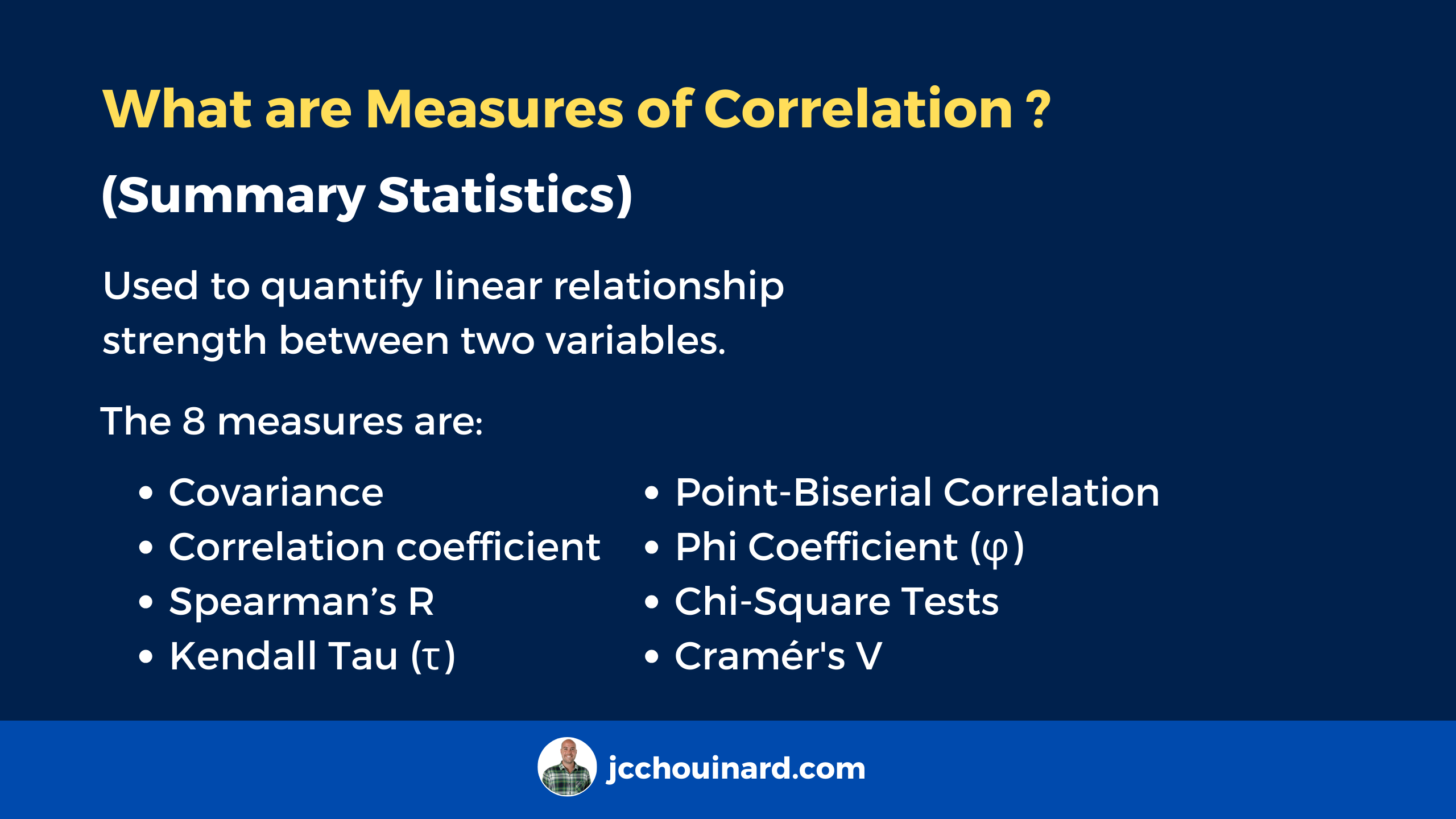
The measures of statistical dependence, also known as the measures of correlation, are the summary statistics used to evaluate the relationships between variables.
The 8 measures of statistical dependence used to evaluate the correlation between multiple variables are:
- Covariance: How much two random variables change together
- Correlation Coefficient: Linear relationship of two continuous variables
- Spearman’s Rank Correlation: Strength/direction of the monotonic relationship between two variables.
- Kendall’s Tau (τ): Strength/direction of ordinal association between two variables.
- Point-Biserial Correlation: Relationship between a continuous and a binary variables
- Phi Coefficient (φ): Association between two binary variables.
- Contingency Tables / Chi-Square Tests: Association between two categorical variables
- Cramér’s V: Association for categorical variables based on chi-square statistics
In this tutorial, we will focus on the most common measures: Covariance, Pearson’s Correlation Coefficient (linear correlation), Spearman’s Rank Correlation (monotonic correlation), and Kendall’s Tau (ordinal correlation).
Covariance
The covariance measures how much two variables change together.
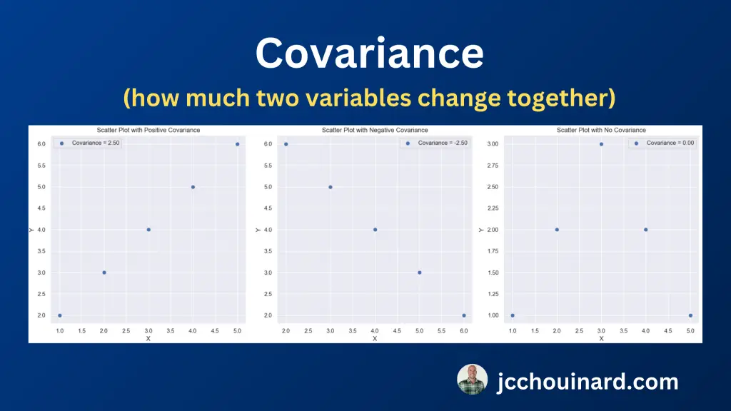
It shows how much a variation in one variable is associated with a variation in another.
The downside of using the covariance in establishing the correlation is that it is sensitive to the scale of the variables.
Calculate the Covariance
To calculate the covariance, you need to get the average from each variable and subtract each value from the average, multiply the matrices and add the values together. Finally, divide the result by the number of values.
The formula of the covariance is
Cov(X, Y) = Σ(Xi-µ)(Yj-v) / nCalculate the Covariance in Python
To calculate the covariance between two array variables in Python, use the cov() function from the numpy library.
import numpy as np

# Sample data
x = np.array([1, 2, 3, 4, 5])
y = np.array([2, 3, 4, 5, 6])

# Calculate the covariance matrix
np.cov(x, y)
The function returns a 2×2 array (or covariance matrix) where diagonal values measure variability and off-diagonal values show relationships.
- Positive means they tend to increase together
- Negative means one goes up when the other goes down.
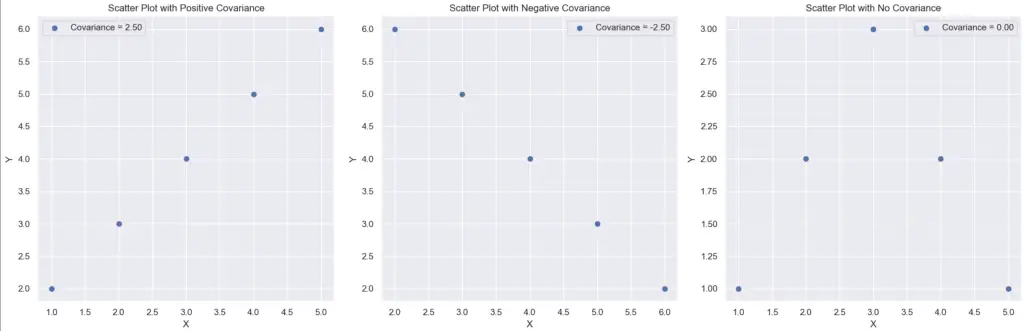
Here are examples of different kinds of covariance matrices.
import numpy as np
# Sample data
x = np.array([1, 2, 3, 4, 5])
x2 = np.array([6, 5, 4, 3, 2])
y = np.array([2, 3, 4, 5, 6])
x3 = np.array([1, 2, 3, 4, 5])
y3 = np.array([1, 2, 3, 2, 1]) # Example with no covariance
# Calculate the covariance matrices
cov_matrix = np.cov(x, y)
cov_matrix2 = np.cov(x2, y)
cov_matrix3 = np.cov(x3, y3)
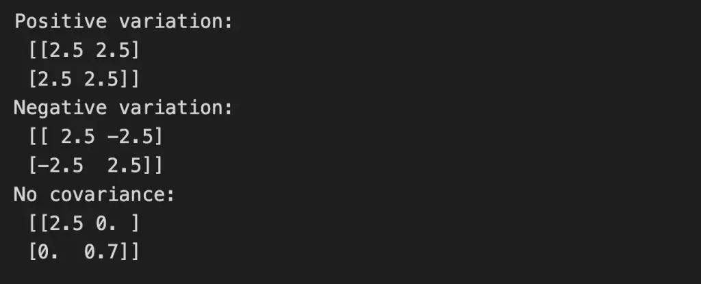
print('Positive variation:\n', cov_matrix)
print('Negative variation:\n', cov_matrix2)
print('No covariance:\n', cov_matrix3)
And what it looks like on a graph
Pearson’s Correlation Coefficient
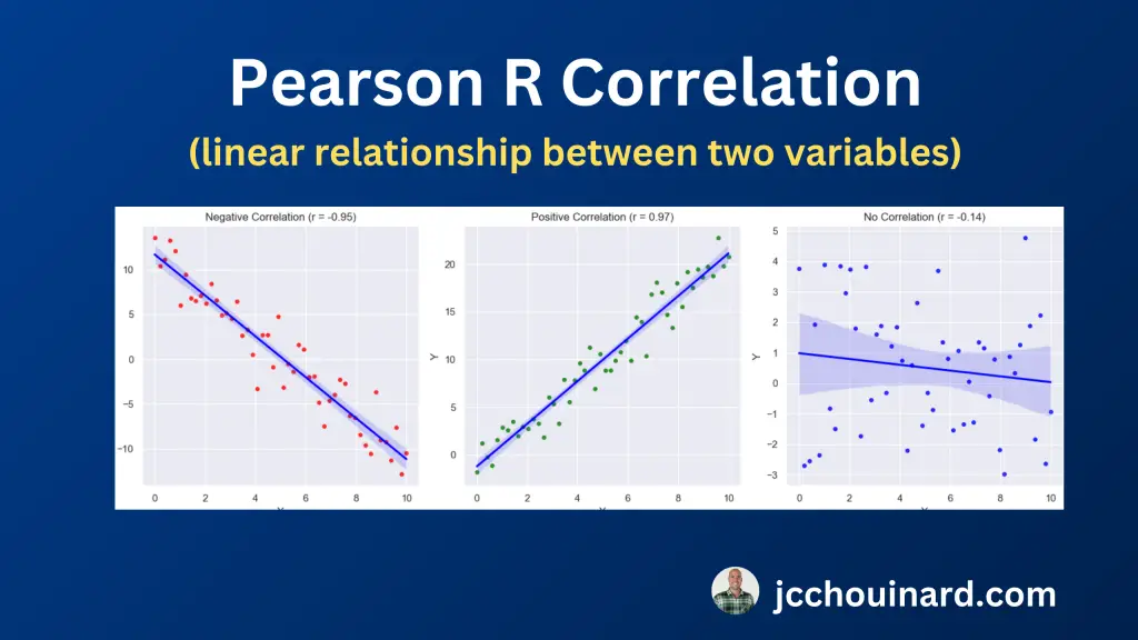
The Pearson’s r correlation coefficient quantifies the linear relationship between two continuous variables.
The results ranges from -1 to 1:
- Perfect negative correlation: -1
- Perfect positive correlation: 1
- No linear Correlation: 0
Calculate Pearson’s R Coefficient in Python
To calculate the Pearson’s R correlation coefficient, use the pearsonr function from scipy.stats library.
import numpy as np
from scipy.stats import pearsonr

# Sample data
x = np.array([1, 2, 3, 4, 5])
y = np.array([2, 3, 4, 5, 6])

# Calculate Pearson's correlation coefficient
correlation_coefficient, _ = pearsonr(x, y)
print("Pearson's Correlation Coefficient:", correlation_coefficient)
The output here shows a perfect positive correlation where when 1 variable increases by one, the other increases by the same amount.
Pearson's Correlation Coefficient: 1.0Plot Pearson’s R Correlation in Python
import numpy as np
import matplotlib.pyplot as plt
from scipy.stats import pearsonr
import seaborn as sns
# Create data for scenarios
np.random.seed(0)
# Negative correlation
x_neg = np.linspace(0, 10, 50)
y_neg = -2 * x_neg + 10 + np.random.normal(0, 2, 50)
# Positive correlation
x_pos = np.linspace(0, 10, 50)
y_pos = 2 * x_pos + np.random.normal(0, 2, 50)
# No correlation
x_no_corr = np.linspace(0, 10, 50)
y_no_corr = np.random.normal(0, 2, 50)
# Calculate Pearson correlation coefficients
corr_coeff_neg, _ = pearsonr(x_neg, y_neg)
corr_coeff_pos, _ = pearsonr(x_pos, y_pos)
corr_coeff_no_corr, _ = pearsonr(x_no_corr, y_no_corr)
# Create subplots
fig, axes = plt.subplots(1, 3, figsize=(15, 5))
# Scatter plot 1 (Negative Correlation)
sns.regplot(x=x_neg, y=y_neg, ax=axes[0], color='red', scatter_kws={'s': 15}, line_kws={'color': 'blue'}, ci=95)
axes[0].set_xlabel('X')
axes[0].set_ylabel('Y')
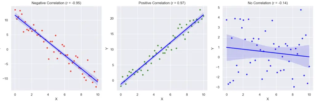
axes[0].set_title(f"Negative Correlation (r = {corr_coeff_neg:.2f})")
# Scatter plot 2 (Positive Correlation)
sns.regplot(x=x_pos, y=y_pos, ax=axes[1], color='green', scatter_kws={'s': 15}, line_kws={'color': 'blue'}, ci=95)
axes[1].set_xlabel('X')
axes[1].set_ylabel('Y')
axes[1].set_title(f"Positive Correlation (r = {corr_coeff_pos:.2f})")
# Scatter plot 3 (No Correlation)
sns.regplot(x=x_no_corr, y=y_no_corr, ax=axes[2], color='blue', scatter_kws={'s': 15}, line_kws={'color': 'blue'}, ci=95)
axes[2].set_xlabel('X')
axes[2].set_ylabel('Y')
axes[2].set_title(f"No Correlation (r = {corr_coeff_no_corr:.2f})")
# Adjust layout
plt.tight_layout()
# Show all plots
plt.show()
Spearman’s Rank Correlation (rho)
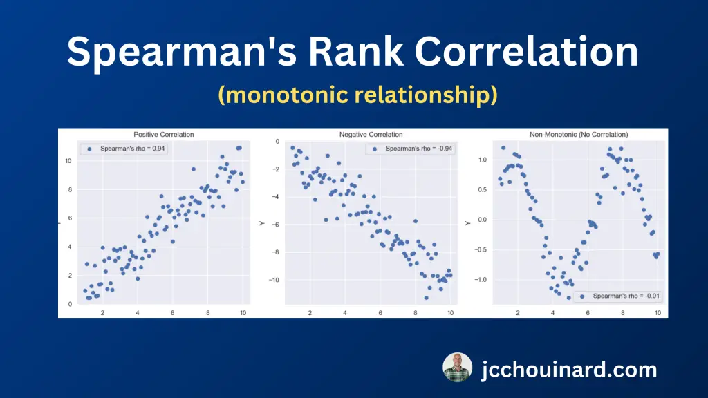
The Spearman’s rank correlation, also known as Spearman’s rho, evaluates the strength and direction of the monotonic relationship between two variables.
A monotonic relationship is a relationship between variables that happens when the value of variable increases or decreases when the other variable increases.
Spearman’s rho check the ranks of the data instead of their actual values. This makes it less impacted by outliers and helps with ordinal data.
Calculate Spearman’s Rank Correlation in Python
To calculate the Spearman’s Rank Correlation, use the spearmanr function from scipy.stats library.
from scipy.stats import spearmanr
# Example data
x = [10, 20, 30, 40, 50]
y = [5, 15, 25, 35, 45]

# Calculate Spearman's rank correlation
rho, p_value = spearmanr(x, y)

# Print the result
print(f"Spearman's Rank Correlation Coefficient: {rho}")
print(f"P-value: {p_value}")
Interpret the Spearman’s Rank Correlation (rho) Result
When interpreting the Spearman’s rho number, check this general guideline:
- Positive rho: As one variable increases, the other tends to increase,
- Negative rho: As one variable increases, the other tends to decrease.
- Rho = 0: No monotonic relationship.
Kendall’s Tau (τ)
In statistics, Kendall’s Tau (τ) measures the strength and direction of the ordinal association between two variables.
Calculate Kendall’s Tau (τ) in Python
To calculate the Spearman’s Rank Correlation, use the kendalltau function from scipy.stats library.
import numpy as np
from scipy.stats import kendalltau

# Sample data
x = np.array([1, 2, 3, 4, 5])
y = np.array([2, 3, 1, 5, 4])

# Calculate Kendall's Tau
tau, p_value = kendalltau(x, y)

print(f"Kendall's Tau (τ): {tau:.2f}")
print(f"P-value: {p_value:.4f}")
Interpret the Kendall’s Tau (τ) Result
When interpreting the Kendall’s Tau (τ) number, check this general guideline:
- τ is close to 1: Strong positive correlation
- τ is close to -1: Strong negative correlation
- τ is close to 0: No correlation
Choose the Right Correlation Metrics (CV, R, Rho or Tau)
Refer to this table to evaluate which correlation algorithm to choose to evaluate the relationship between variables.
| Correlation Measure | Best for Data Type | Robust to Outliers | Type of Relationship |
|---|---|---|---|
| Covariance | Interval Data, Ratio Data | No | Linear |
| Pearson’s Correlation Coefficient (r) | Interval Data, Ratio Data | No | Linear |
| Spearman’s Rank Correlation (ρ) | Ordinal Data, Interval Data | Yes | Monotonic |
| Kendall’s Tau (τ) | Ordinal Data, Data with Tied Ranks | Yes | Concordance or Discordance |

SEO Strategist at Tripadvisor, ex- Seek (Melbourne, Australia). Specialized in technical SEO. Writer in Python, Information Retrieval, SEO and machine learning. Guest author at SearchEngineJournal, SearchEngineLand and OnCrawl.