In this guide, we will introduce one of the summary statistics: the measures of variability. We will also provide you with Python examples to illustrate how to apply this concept.
What are the Measures of Variability (Spread) in Statistics
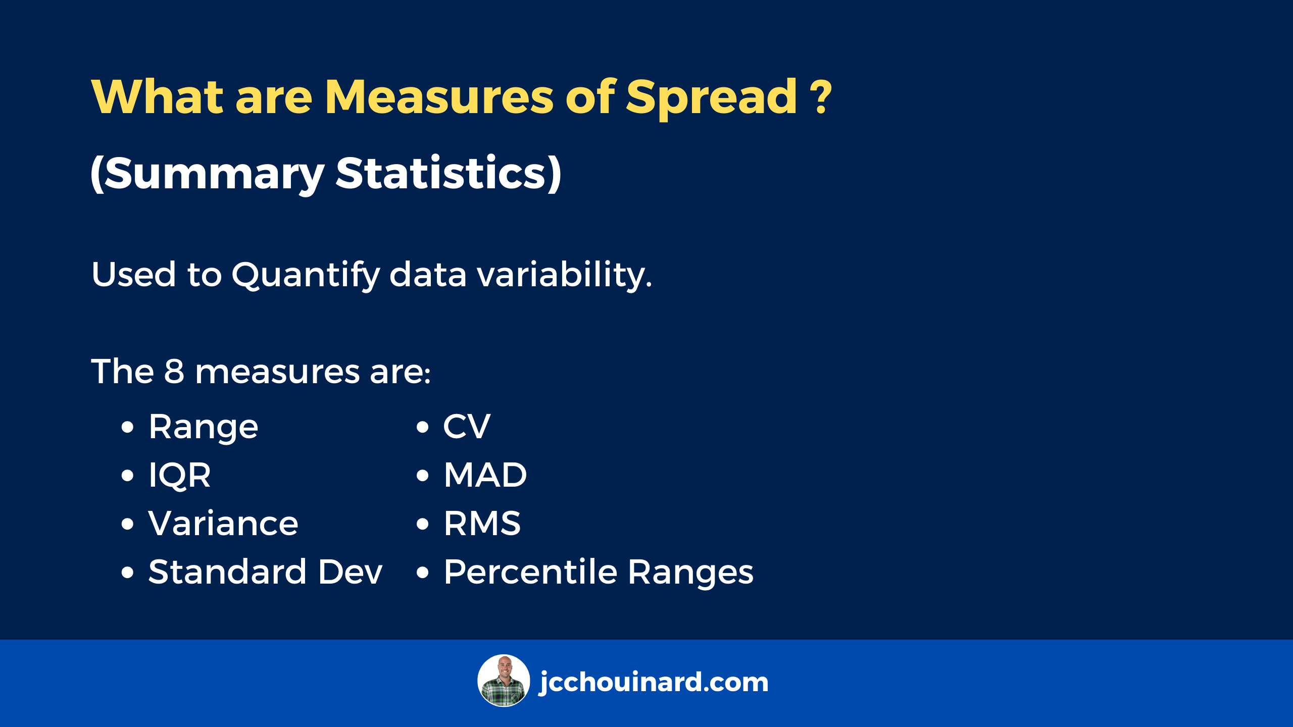
The measures of variability, also known as measures of spread, are. the summary statistics used to understand the variability of the data how close or spread apart the data points are).
The 8 measures of variability in summary statistics are the range, the interquartile range (IQR), the variance, the standard deviation, the Coefficient of Variation (CV), the Mean Absolute Deviation, the Root Mean Square (RMS) and the Percentile Ranges.
- Range: Difference between the maximum and minimum values in a dataset
- Interquartile Range (IQR): Difference between the third and first quartiles (Q3 and Q1) . Focuses on the middle 50% to reduce the impact of outliers.
- Variance: Average distance of each data point from the mean
- Standard Deviation: Square-root of the variance
- Coefficient of Variation (CV): Percentage ratio of the standard deviation to the mean
- Mean Absolute Deviation: Average absolute difference between data points and the mean
- Root Mean Square (RMS): Square root of the mean of the squared values.
- Percentile Ranges: Ranges between specific percentiles to provide insights into the central of the data less influenced by extreme values.
Overview of Measures of Variability in Python
| Name | Description | When to Use | Python Function |
|---|---|---|---|
| Range | Difference between max and min. | Quick overview of spread. | max(data) - min(data) |
| Interquartile Range (IQR) | Range of middle 50% data. | Robust to outliers. | np.quantile(data, 0.75) - np.quantile(data, 0.25) |
| Variance | Average squared deviations. | Sensitive to outliers. | np.var(data) |
| Standard Deviation | Square root of variance. | Interpretable, in same units. | np.std(data) |
| Coefficient of Variation (CV) | Standard deviation relative to mean. | Comparing datasets with different scales. | (np.std(data) / np.mean(data)) * 100 |
| Mean Absolute Deviation (MAD) | Average absolute deviations. | Robust to outliers. | np.mean(np.abs(data - np.mean(data))) |
| Root Mean Square (RMS) | Square root of mean of squared values. | Used in signal processing. | np.sqrt(np.mean(np.square(data))) |
| Percentile Ranges | Ranges between specific percentiles. | Highlight central data range. | numpy.percentile(data, q) - numpy.percentile(data, p) |
What is the Range in Statistics
The Range in statistics represents the difference between the maximum and minimum values of a dataset.
How to Calculate the Range
The range is calculated by subtracting the minimum value from the maximum value.
range = max - minHow to Calculate the Range in Python
To calculate the range for values in Python, use the max() and the min() function. Note that the range() function is used to create the range, not to calculate it.
values = range(1, 10) # create range
rg = max(values) - min(values) # calculate range

print('Values:', list(values))
print('Range:', rg)
Values: [1, 2, 3, 4, 5, 6, 7, 8, 9]
Range: 8
What is the Interquartile Ranges (IQR) in Statistics
The Interquartile Ranges, or IQR, in summary statistics represents the difference between the third quartile (Q3) and the first quartile (Q1). By focusing on the middle 50% of the data, the Interquartile Ranges allow an analysis that is less influenced by extreme values.
Simply put, the interquartile range is the height of the box in a boxplot.

To understand IQR, we need to introduce the concept of quantiles.
What are Quantiles (Percentiles) in Statistics
Quantiles, also known as percentiles, occurs when we split the data in equal parts. For example, when we split quantiles into 4 equal parts, we call those quartiles.
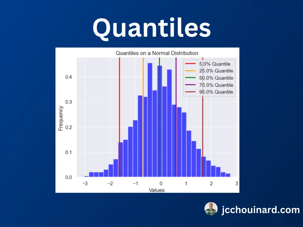
We can use the np.quantile() function in Python to split the data in equal parts.
import numpy as np

# Example numerical dataset
data = np.array(range(1,10))

# Calculate the median (50th percentile)
median = np.quantile(data, 0.5)
print("Median (50th percentile):", median)

np.median(data) == np.quantile(data, 0.5)
Median (50th percentile): 5.0
True
You can see how, in the code above, quantiles split in 50% is the same as computing the median value.
You can also calculate the 25th, 75th and 90th percentiles of your dataset.
# Calculate the 25th percentile (1st quartile)
q1 = np.quantile(data, 0.25)
print("25th Percentile (1st Quartile):", q1)

# Calculate the 75th percentile (3rd quartile)
q3 = np.quantile(data, 0.75)
print("75th Percentile (3rd Quartile):", q3)

# Calculate a custom quantile (e.g., the 90th percentile)
custom_quantile = np.quantile(data, 0.9)
print("90th Percentile (Custom Quantile):", custom_quantile)

# Calculate all quartiles at once
quartiles = np.quantile(data, [0,0.25,0.5,0.75,1])
print("Quartiles:", quartiles)
25th Percentile (1st Quartile): 3.0
75th Percentile (3rd Quartile): 7.0
90th Percentile (Custom Quantile): 8.2
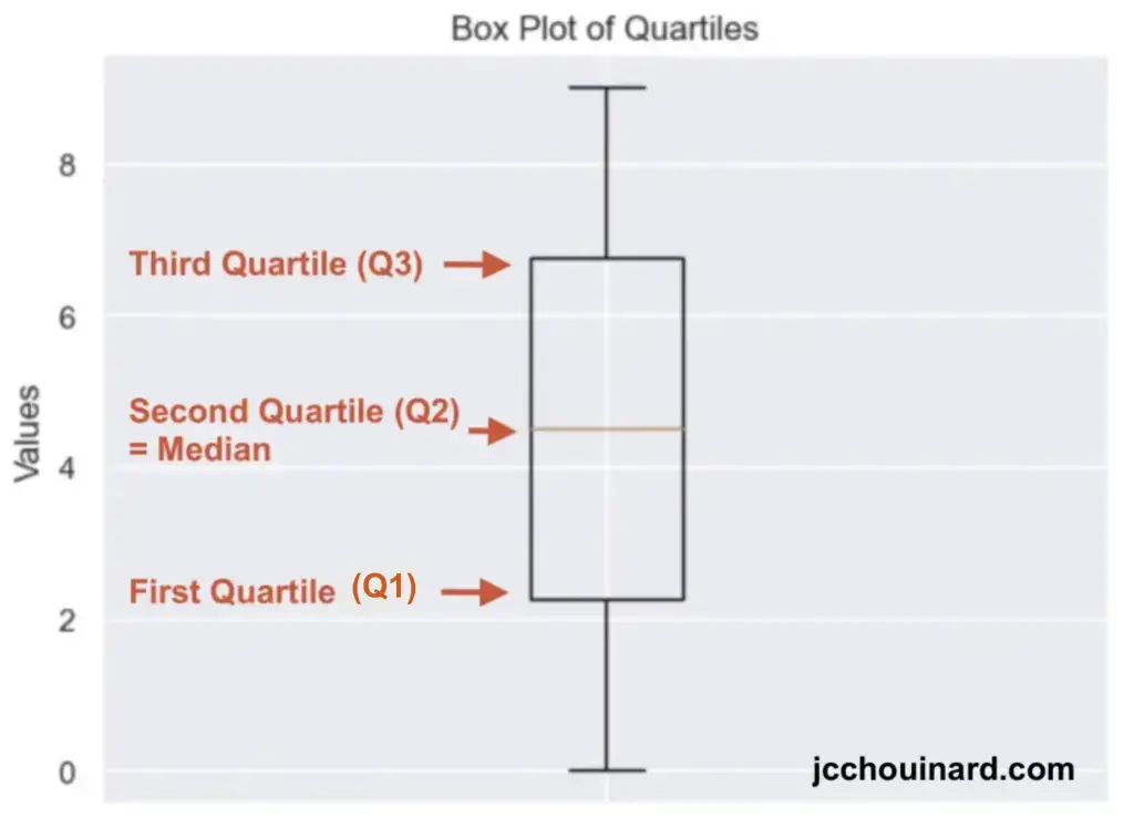
Quartiles: [1. 3. 5. 7. 9.]Visualize Quantiles with a Box Plot in Python
The best way to visualize quantiles in Python, is to create a box plot from your data.
import matplotlib.pyplot as plt
import numpy as np

# Example numerical dataset
data = np.array(range(10))

# Create a box plot
plt.boxplot(data)

# Add labels and a title
plt.xlabel("Dataset")
plt.ylabel("Values")
plt.title("Box Plot of Quartiles")

# Show the plot
plt.show()
How to Calculate the Interquartile Ranges
The interquartile range is calculated by subtracting quartile 1 data from quartile 3 data.
IQR = Q3(data) - Q1(data)How to Calculate the Interquartile Ranges in Python
The interquartile ranges (IQR) can be calculated in Python by using np.quantiles() to subtract the first quantile from the third, or by using the iqr() function from the scipy.stats module.
With np.quantile
np.quantile(data, 0.75) - np.quantile(data, 0.25)With Scipy.stats
from scipy.stats import iqr

iqr(range(1,10))
4.0What is the Variance in Statistics
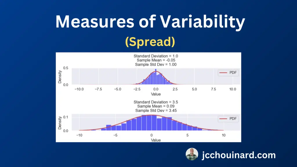
The variance in statistics is a measure of the spread or variability of a dataset.
The variance quantifies how far individual data points in a dataset differ from the mean (average) of the dataset.
Simply put, the variance show how dispersed or scattered the data points are around the mean.
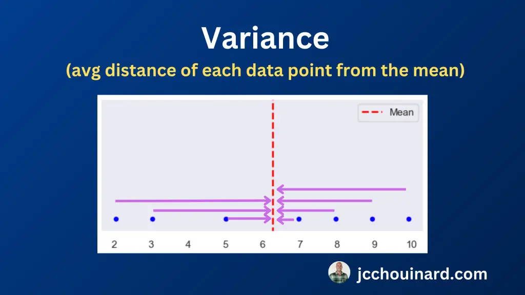
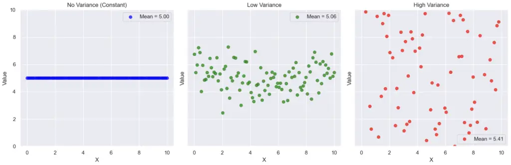
On a scatter plot, we can easily visualize the dispersion of the data by modifying the variance.
How to Calculate the Variance
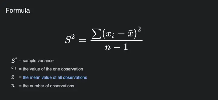
To calculate the variance, subtract the mean from each data point, square the distances, sum all the squared values and divide by the number of data points minus 1.
Formula of the variance
How to Calculate the Variance in Python
To compute the variance in Python, either use the var() function from numpy or compute the sum the squared distances from the mean and divide by the number of values minus 1.
Calculate the variance with Python Numpy
To calculate the variance in Python with Numpy, use the var() function with the ddof argument set to 1. The ddof argument is used to specify the formula to use when working with a sample of data.
# Variance with np.var()
import numpy as np

data_points = [1,2,3,4,5]
np.var(data_points, ddof=1)
Calculate the variance manually with Python
Follow these steps to calculate the variance manually in Python:
- Calculate distances from the mean
- Square the distances
- Sum the squared distances
- Find Number of data points
- Divide the sum of the squared distances by n-1
import numpy as np

data_points = [1,2,3,4,5]


# 1. Calculate distances from the mean
distances = data_points - np.mean(data_points)
print('1. Mean distances:', distances)

# 2. Square the distances
sqr_distances = distances ** 2
print('2. Squared distances:', sqr_distances)

# 3. Sum the squared distances
summed_distances = sum(sqr_distances)
print('3. Sum of the squared distances:', summed_distances)

# 4. Find Number of data points
n = len(data_points)
print('4. Number of data points:', n)

# 5. Divide the sum of the squared distances by n-1
variance = summed_distances / (n - 1)
print('5. Variance:', variance)
Output
1. Mean distances: [-2. -1.  0.  1.  2.]
2. Squared distances: [4. 1. 0. 1. 4.]
3. Sum of the squared distances: 10.0
4. Number of data points: 5
5. Variance: 2.5
Note that the S^2 notation shows how the result of the variance is a squared value on which the sqare-root could be applied to compute the standard deviation.
What is the Standard Deviation in Statistics
The standard deviation in statistics is a measure of the spread or variability of a dataset calculated using the square-root of the variance.
Simply put, the standard deviation is the square-root of the variance.
The advantage of the standard deviation compared to the variance is that the standard deviation is in the same units as your data points (seconds, minutes, days, etc.).
How to Calculate the Standard Deviation
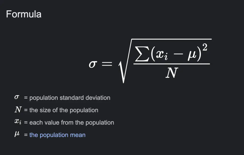
To calculate the standard deviation, calculate the variance and compute the square-root of the variance.
Formula of the standard deviation
How to Calculate the Standard Deviation in Python
To compute the standard deviation in Python, either use the std() function from numpy or use the np.sqrt() function on the computed variance.
np.std(data_points)np.sqrt(np.var(data_points))Just note that using the np.std() function will compute the sqrt() function on the variation calculated from a division with n, not n-1.
import numpy as np

data_points = [1,2,3,4,5]
# Standard deviation with np.std
print('std():',np.std(data_points))

# Standard deviation with np.sqrt(np.var()) n
variance = np.var(data_points)
print('np.sqrt(np.var()):',np.sqrt(variance))
# Standard deviation with np.std
print('std(ddof=1):',np.std(data_points, ddof=1))

# Standard deviation with np.sqrt(np.var()) n-1
variance = np.var(data_points, ddof=1)
print('np.sqrt(np.var(ddof=1)):',np.sqrt(variance))
Output
std(): 1.4142135623730951
np.sqrt(np.var()): 1.4142135623730951

std(ddof=1): 1.5811388300841898
np.sqrt(np.var(ddof=1)): 1.5811388300841898
What is the Coefficient of Variation (CV) in Statistics
The Coefficient of Variation, or CV, in statistics is a a relative measure of variability represented by the percentage ratio of the standard deviation and the mean.
How to Calculate the Coefficient of Variation
To calculate the coefficient of variation (CV), you need to calculate the standard deviation and the mean of a dataset. Then, find the coefficient of variation by computing the ration of the standard deviation to the mean.
cv = (std/mean) * 100How to Calculate the Coefficient of Variation in Python
To calculate the coefficient of variation in Python, use the mean() and the std() function of the numpy library, and then divide the standard deviation by the mean.
import numpy as np

# Sample data
data_points = [1, 2, 3, 4, 5]

# Calculate the mean (average) of the data
mean = np.mean(data_points)

# Calculate the standard deviation of the data
std_dev = np.std(data_points)

# Calculate the Coefficient of Variation (CV)
cv = (std_dev / mean) * 100

# Print the result
print(f"Coefficient of Variation (CV): {cv:.2f}%")
Coefficient of Variation (CV): 47.14%What is the Mean Absolute Deviation in Statistics
The Mean Absolute Deviation, or MAD, in statistics is the average absolute difference between data points and the mean. It is often used as an alternative to the standard deviation since it does not require to square deviations.
How to Calculate the Mean Absolute Deviation
To calculate the mean absolute deviation, calculate the differences between each data point and the mean. Then, get the absolute values. Finally, compute the mean.
mad = mean(absolute(data_points - mean(data_points)))How to Calculate the Mean Absolute Deviation in Python
To calculate the mean absolute deviation (MAD) in Python, get the absolute values from the subtraction of the mean from each data point, then find out the mean of the absolute values.
import numpy as np

data_points = [1,2,3,4,5]

# 1. Calculate distances from the mean
distances = data_points - np.mean(data_points)
print('1. Mean distances:', distances)

# 2. Calculate the mean absolute deviation
mad = np.mean(np.abs(distances))
print('2. Mean absolute deviation:', mad)
1. Mean distances: [-2. -1.  0.  1.  2.]
2. Mean absolute deviation: 1.2
What is the Root Mean Square (RMS) in Statistics
The Root Mean Square, or RMS, in statistics represents the square root of the mean of the squared values used to measure the magnitude of variations.
How to Calculate the Root Mean Square
Mathematically, the RMS can be represented as:
RMS = sqrt((x₁² + x₂² + ... + xₙ²) / n)How to Calculate the Root Mean Square in Python
To calculate the root mean square in Python,
- Square each data point in your dataset.
- Calculate the mean of the squared values
- Take the square root the mean of the squared values.
import numpy as np

# Sample data
data_points = [1, 2, 3, 4, 5]

# 1. Square each value
squared_data = [x**2 for x in data_points]

# 2. Find the mean of the squared values
mean_squared = np.mean(squared_data)

# 3. Take the square root
rms = np.sqrt(mean_squared)

print(f"Root Mean Square (RMS): {rms}")
Root Mean Square (RMS): 3.3166247903554What is the Percentile Ranges in Statistics
The Percentile Ranges is a summary statistic extracted using the ranges between specific percentiles (e.g 10th and 90th percentiles). The percentile ranges provide insights into the central X% of the dat, which is less influenced by outliers.
How to Calculate the Percentile Ranges in Python
Calculating percentile ranges in Python is similar to calculating interquartile ranges, but with custom percentiles specified. You can do so by using the percentile() function of the numpy library.
# Calculate the first percentile (Q1)
q1 = np.percentile(sorted_data, 25)

# Calculate the third percentile (Q3)
q3 = np.percentile(sorted_data, 75)

# Calculate the percentile range
percentile_range = q3 - q1
Outliers
Outliers in statistics are the extreme data points that are significantly different from the others. They can have a big impact on the measures of variability and should be understood, and dealt with accordingly, by statistician and data scientists. Check out our tutorial to understand how to identify outliers in a dataset.

SEO Strategist at Tripadvisor, ex- Seek (Melbourne, Australia). Specialized in technical SEO. Writer in Python, Information Retrieval, SEO and machine learning. Guest author at SearchEngineJournal, SearchEngineLand and OnCrawl.