I decided to create a daily post for 30 days about Pandas to show why I love this library. Here I would give method and function I deemed useful and interesting enough. Let’s just get into it.
If you want to get an overview first, you can look at Pandas functions to replace Excel.
Day 1: style.bar
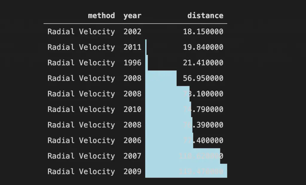
I want to showcase a method from Pandas Data Frame Object called style.bar which allowed you to create a barplot of numerical column inside your Data Frame. You only need to call this method by using the .style.bar after the Data Frame object.
This method is useful if you want to give more impact to your data presentation and specify your point more clearly.
import pandas as pd
import seaborn as sns

planets = sns.load_dataset('planets')

planets.head(10)[['method','year', 'distance']].sort_values(by = 'distance').style.bar(color = 'lightblue',
                                                                                       subset = 'distance').hide_index()
Day 2: qcut
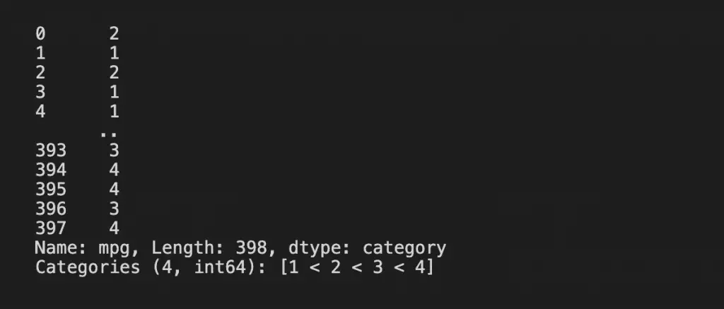
Today, I want to show you a useful function from pandas to dividing your data called qcut.
What is Pandas Function qcut? qcut function would bin the continuous variable where the bin size would be equal-sized based on rank or based on sample quantile.
So what is quantile? quantile is basically a division technique to divide the continuous value in an equal way. For example, if we divide the continuous value into 4 parts; it would be called Quartile as shown in the picture.
import seaborn as sns
import pandas as pd
mpg = sns.load_dataset('mpg')

pd.qcut(x = mpg['mpg'], q = 4, labels = [1,2,3,4])
Day 3: pivot_table
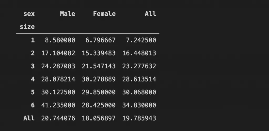
In this post, I want to introduce you to one of the most powerful methods called pivot_table.
This method could be accessed in the data frame object by calling the method .pivot_table after the Data Frame object.
So what is this method do? It creates a pivot table based on the categorical object we passed on the columns parameter with the values parameter accepting numerical values.
What special about pivot_table is that the result is not just the values but the aggregate function passed on the parameter.
You could look at the example picture for more information. I hope it helps!
import pandas as pd
import seaborn as sns
tips = sns.load_dataset('tips')

tips.pivot_table(columns = 'sex', values = 'total_bill', aggfunc = 'mean', index = 'size', margins = True)
Day 4: agg
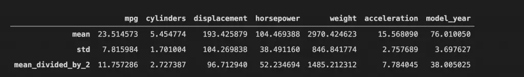
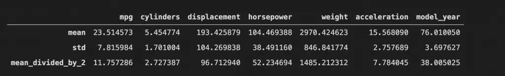
Let’s start with an easier method today. Here, I want to introduce a method from the Data Frame object called agg.
Just like the name, this method creates an aggregation table. It means, we put our intended aggregation in the .agg method and all the numerical columns are processed by the aggregation function which creates the table.
What is great about this function is that we could put our intended aggregation ourselves by creating our function and the resulted table would be shown just like in the example picture.
import pandas as pd
import seaborn as sns

mpg = sns.load_dataset('mpg')

def mean_divided_by_2(col):
    return (col.mean())/2

mpg.agg(['mean', 'std',mean_divided_by_2])
Day 5: melt
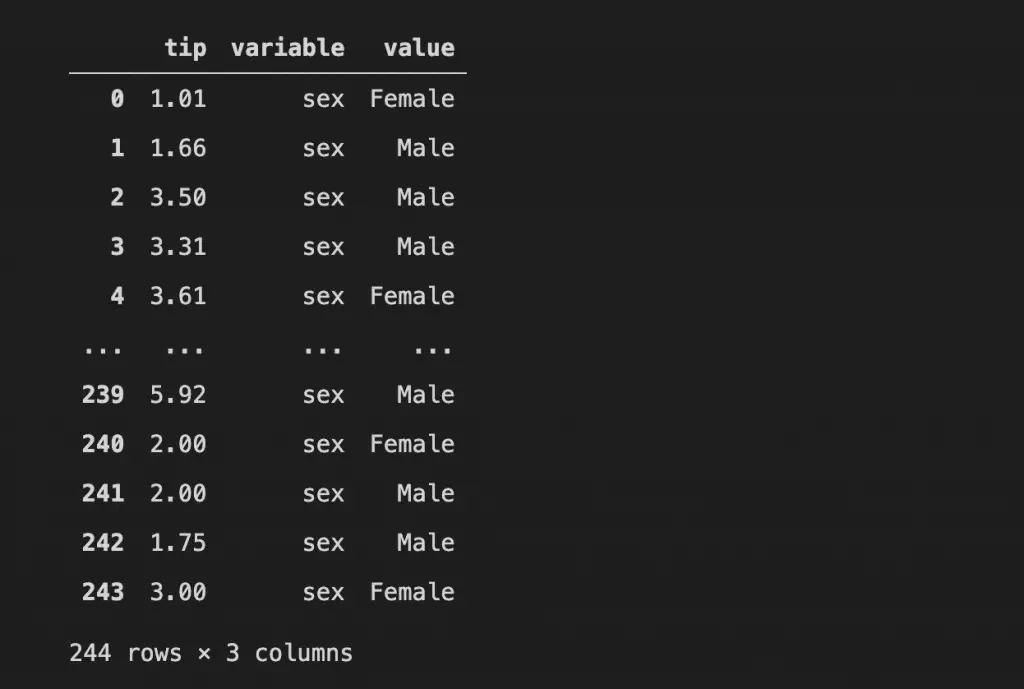
I want to introduce you to a peculiar method from pandas Data Frame called melt.
This method is a reverse from the pivot method when we break down every value and variable to another table.
Just look at the example below, this time I specify the id_vars as a tip column and the value is the sex column. What we get is every value from the tip column and every value from the sex column is paired.
import pandas as pdimport seaborn as snstips = sns.load_dataset('tips')
tips.melt(id_vars = 'tip', value_vars = 'sex')
Day 6: style.applymap
Today, I want to introduce you to an exciting method from Pandas Dataframe called style.applymap.
So what is this method do? Well, take a look at the example and you can see some numbers are colored red while others are black. This is happening because we use the style.applymap method.
What this method do is accepting a function to modifying the CSS in our Jupyter Notebook and applied to each and every single value in our Data Frame.
For example, in my example, the function would color the numerical value below and equal to 20. What the function needs to return for each value to change the color is a string with the color specification; e.g. ‘color:red‘.
import pandas as pd
import seaborn as sns

mpg = sns.load_dataset('mpg')

def mean_divided_by_2(col):
    return (col.mean())/2

mpg.agg(['mean', 'std',mean_divided_by_2])
Day 7: select_dtypes
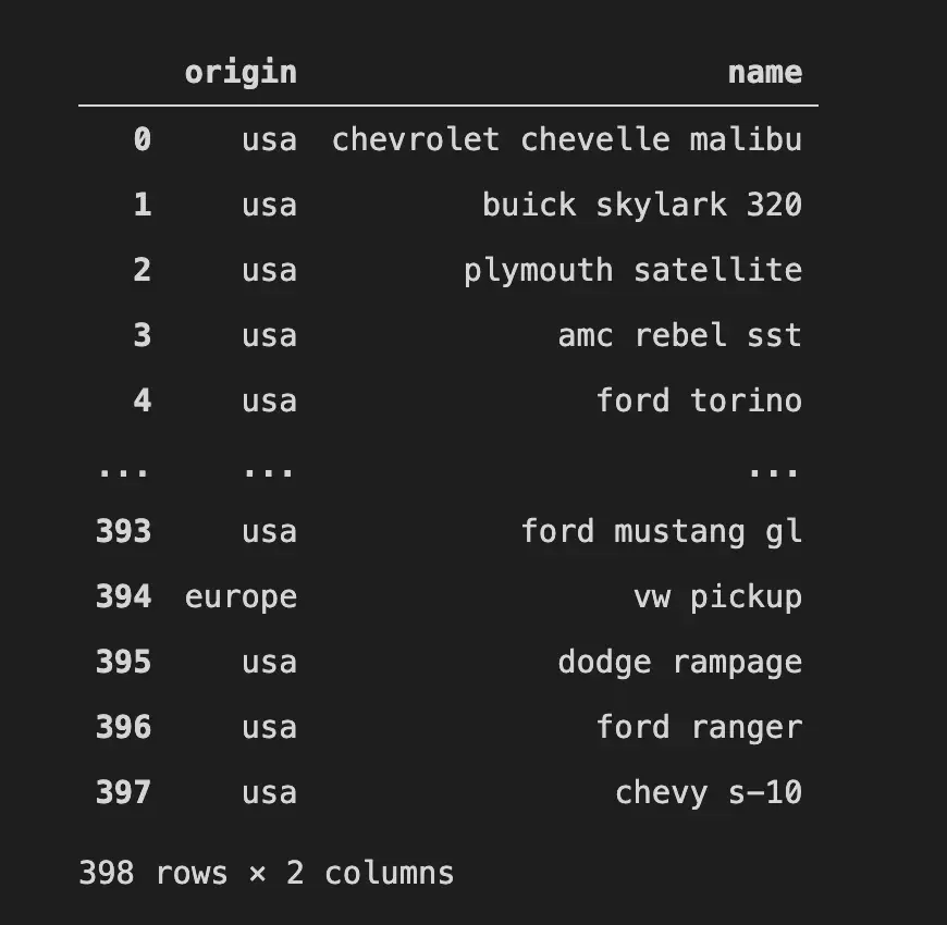
I want to share a simple yet powerful method from Pandas Data Frame called .select_dtypes.
During data cleansing and engineering, I often use this method and would have a hard time without .select_dtypes method.
So, what is this method did? It is simple, this method is used to select the columns in our Data Frame based on the specific data type. For example ‘number’ or ‘object’.
In the example, I showed you I pass ‘number’ data type to the method; this means I only selecting the numerical columns (either float or integer). The other example I use is ‘object’ which means I selecting only the object columns.
import seaborn as sns
import pandas as pd
mpg = sns.load_dataset('mpg')

#Selecting the number data type
mpg.select_dtypes('number')

#Selecting the object data type
mpg.select_dtypes('object')
Day 8: style.hide_
import seaborn as sns
import pandas as pd
mpg = sns.load_dataset('mpg')

mpg.head(10).style.hide_index().hide_columns(['mpg', 'name', 'model_year'])
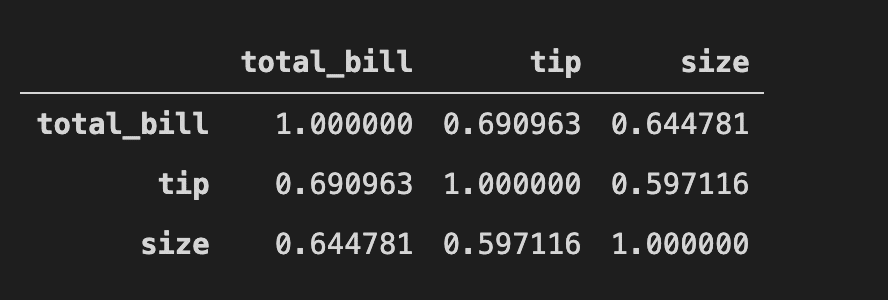
Day 9: corr
import pandas as pd
import seaborn as sns
from scipy.stats import weightedtau

def weight_tau(x, y):
    return weightedtau(x, y)[0]

tips= sns.load_dataset('tips')
tips.corr(weight_tau)
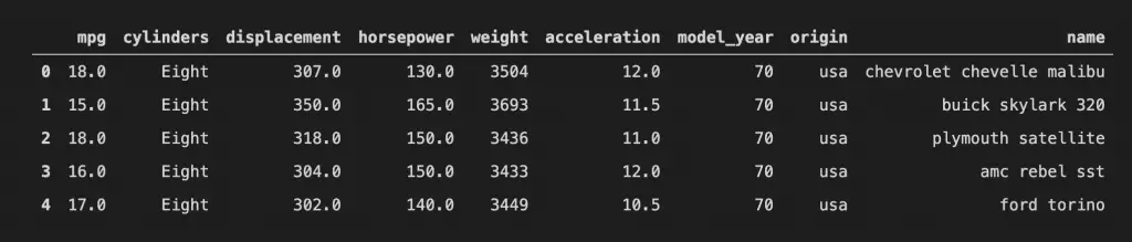
Day 10: replace
Today, I want to introduce you to the Data Frame object method called .replace.
So, this method is just like what the name implies; it used to replace something, but what?
The main things that this method does are to replace values; yes, values within columns.
From the example, you could see that I replace the value by passing a dictionary object within the method. So the logic in my example is: {columns name: {values you want to replace: values to replace}}.
import pandas as pd
import seaborn as sns

mpg = sns.load_dataset('mpg')
mpg.replace({'cylinders' : {3: 'Three', 4: 'Four', 5: 'Five', 6: 'Six', 8 : 'Eight'}}, inplace = True)
mpg.head()
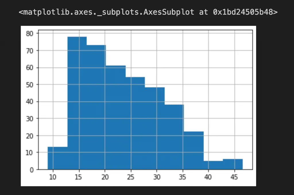
Day 11: hist
Well, I want to introduce you to a cool method from the Pandas Series object called .hist.
So, this method work is simple; It creates a histogram plot from your numerical series object. Simple, right?
You only need to call it and it automatically creates your histogram plot just like in the example.
import seaborn as sns
import pandas as pd
mpg = sns.load_dataset('mpg')

mpg['mpg'].hist()
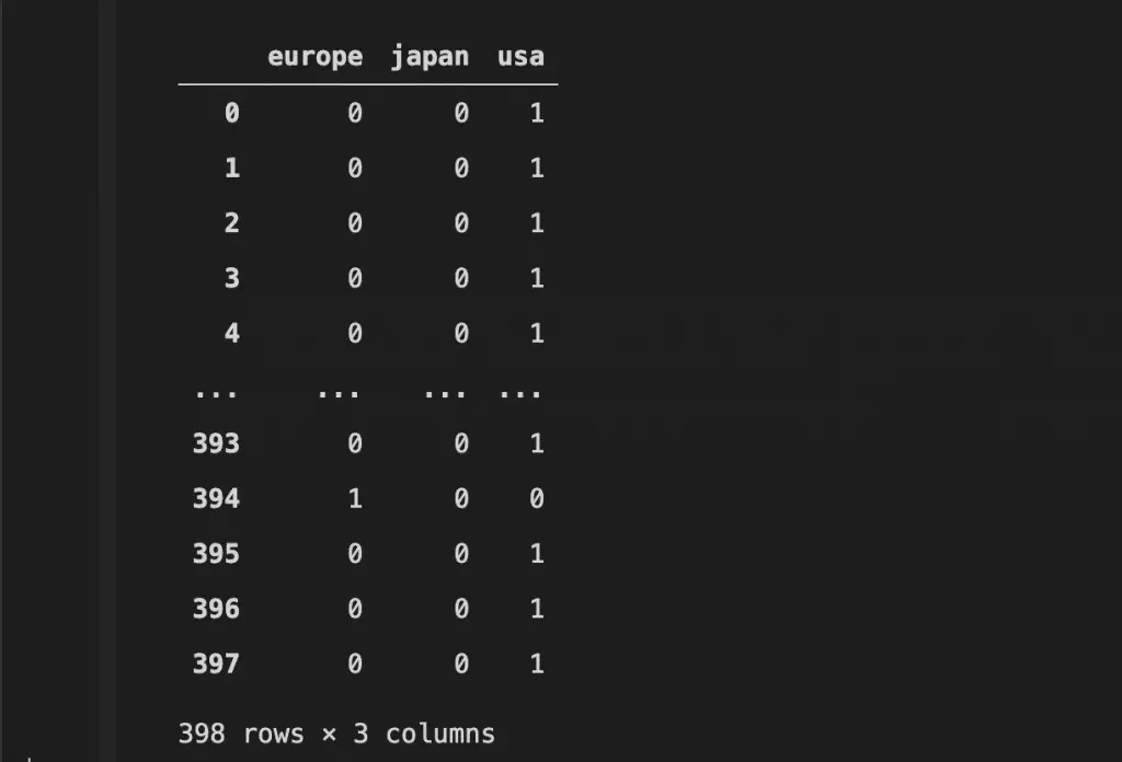
Day 12: get_dummies
I want to introduce you to a special function from Pandas called get_dummies.
From the example, you might get what it does, but for you doesn’t; this method is more known as One Hot Encoding or OHE.
The get_dummies function is used to create new features based on the categorical class in one variable with the value of the new features is 0 or 1; 0 mean not present, 1 mean present.
One Hot Encoding mostly used when you need to transform your categorical data into numerical.
import pandas as pd
import seaborn as sns

mpg = sns.load_dataset('mpg')
pd.get_dummies(mpg['origin'])
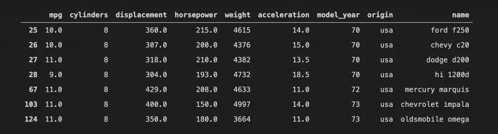
Day 13: query
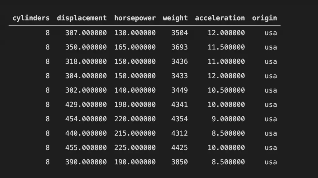
I want to introduce you to a cool Data Frame Method called .query.
So, what is this method do? Well, this method allows selection using a string expression. What is it means?
Look at the example picture, it is like some selection with conditions right? It is a boolean based selection method. after all.
In the example table, we often need to specify the condition to selection like mpg[(mpg['mpg'] <=11) & (mpg['origin] == 'usa')], but with query it was all simplified. Just pass a string condition to the method and we get the same selection result.
import pandas as pd
import seaborn as sns

mpg = sns.load_dataset('mpg')
mpg.query("mpg <= 11 & origin == 'usa'")
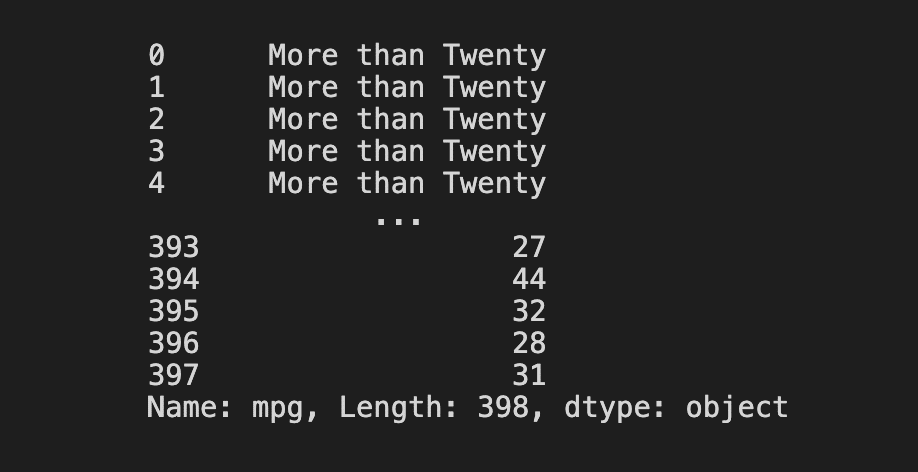
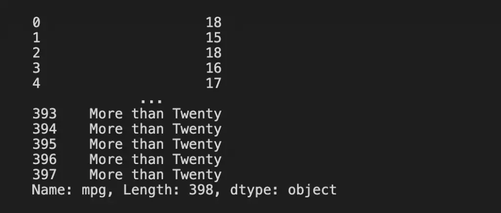
Day 14: mask
I want to introduce you to an if-then method called .mask.
So what is this method do? It is used to replace specific values with another value that meets the condition given.
Let’s see in my example, I pass a condition where the values of the mpg are less than 20 then replace it with ‘More than Twenty’. How cool is that!
import pandas as pd
import seaborn as sns

mpg = sns.load_dataset('mpg')
mpg['mpg'].mask(mpg['mpg'] < 20, 'More than Twenty' )
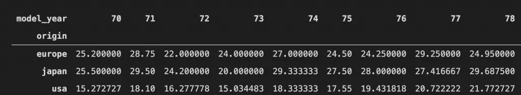
Day 15: crosstab
Halfway there, and so today I want to introduce you to a table formatting function called crosstab.
So, what is this function do? this function would help us to create a pivot table of categorical classes with an aggregation function of a numerical column as the values, although you could also create a count between categorical classes as well.
Look at the example, you could see I specify the origin and model_year (both are categorical) as the index and column respectively. In addition, I make the mpg column as the numerical values and using the mean as the aggregation function.
import pandas as pd
import seaborn as sns

mpg = sns.load_dataset('mpg')
pd.crosstab(index = mpg['origin'], columns = mpg['model_year'], values = mpg['mpg'], aggfunc = 'mean' )
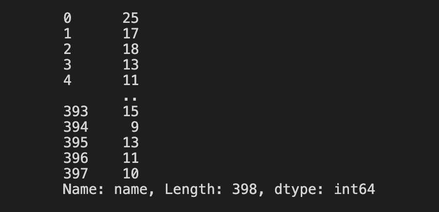
Day 16: apply
The apply pandas method is a method that I use so often during my analysis time, I become accustomed to how neat it is. The Pandas Data Frame method is .apply.
This method accepting a function and applied it to the whole data (either in row ways or columns way). What the function return is the result.
Just look at the example, I am applying a lambda function which returns the length of each data value.
import pandas as pd
import seaborn as sns

mpg = sns.load_dataset('mpg')
mpg['name'].apply(lambda x: len(str(x)))
Day 17: set_option
import pandas as pd
import seaborn as sns
pd.set_option('display.max_columns', None)
pd.set_option('display.max_rows', 50)

mpg = sns.load_dataset('mpg')
mpg
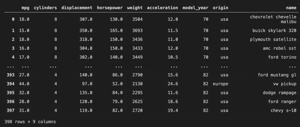
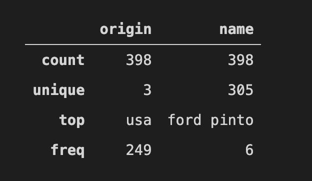
Day 18: describe
I just want to show you to one of the most known method from Pandas Data Frame Object called .describe.
I am betting that most people who start their journey in data science with Python know about this method. For you who does not, this method is a method which produces a Data Frame with all the basic statistic.
Although, there is a little trick in this API. By default, describe only calculate all the numerical columns which in turn giving you information such as the mean, std, percentiles, etc.
However, if you exclude the numerical columns like in the sample, you would end up with a different Data Frame. This time, the non-numerical column would be calculated. Here, what we get are the frequency and top classes.
import pandas as pd
import seaborn as sns

mpg = sns.load_dataset('mpg')

#Describe numerical columns
mpg.describe()

#Describe non-numerical columns
mpg.describe(exclude = 'number')
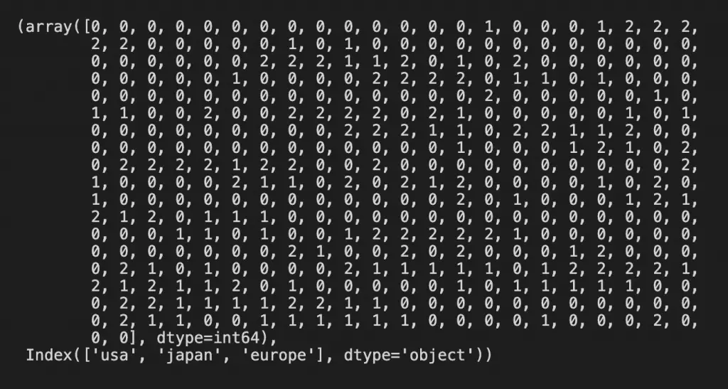
Day 19: factorize
I want to introduce you to one of the useful pandas function and the series method called factorize.
Take a look at the example first, here I take the categorical variable origin and using the factorize method on it. What is the result? There are 2 things, the numerical array and the unique classes.
So what is special about this method? The numerical array you just see is the classes in the categorical variable encoded as a numerical value. How to know which number represents what class? That is why we also get unique classes.
In the sample below 0 is usa, 1 is japan, and 2 is europe. Just like the unique position.
This function is most useful when you need to encode the categorical into numerical values, but when there is an ordinal assumption in there.
import pandas as pd
import seaborn as sns

mpg = sns.load_dataset('mpg')
mpg['origin'].factorize()
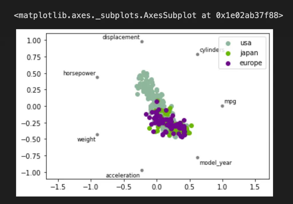
Day 20: plotting.radviz
On the 20th day, I want to introduce a plotting function from Pandas called pd.plotting.radviz.
So, what is this function do? According to Pandas, radviz allows us to project an N-dimensional data set into a 2D space where the influence of each dimension can be interpreted as a balance between the influence of all dimensions.
In a simpler term, it means we could project a multi-dimensional data into a 2D space in a primitive way.
Each Series in the DataFrame is represented as an evenly distributed slice on a circle. Just look at the example, there is a circle with the series name.
Each data point is rendered in the circle according to the value on each Series. Highly correlated Series in the DataFrame are placed closer on the unit circle.
To use the pd.plotting.radviz, you need a multidimensional data set with all numerical columns but one as the class column (should be categorical).
import pandas as pd
import seaborn as sns

mpg = sns.load_dataset('mpg')
pd.plotting.radviz(mpg.drop(['name'], axis =1), 'origin')
Day 21: scatter_matrix
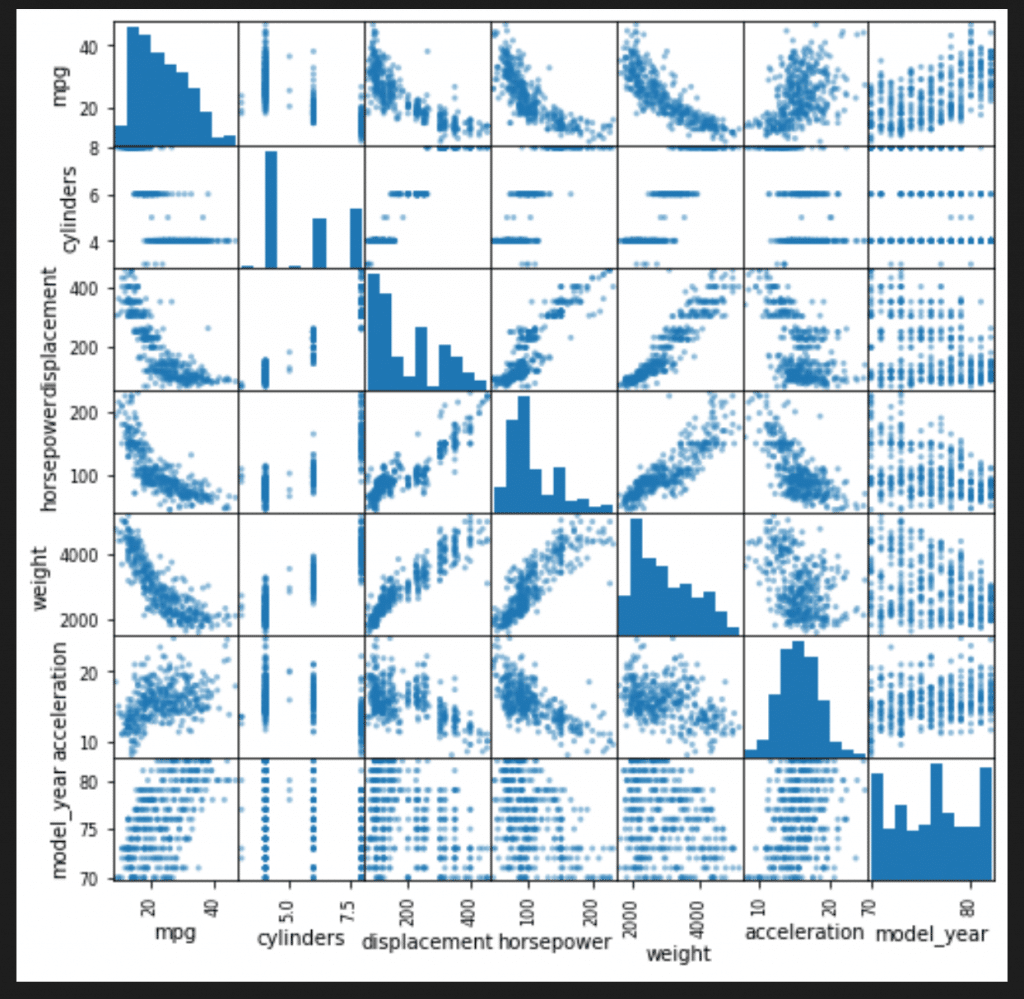
Today is another plotting function of Pandas that I want to introduce. This time, the function is called plotting.scatter_matrix.
This is a simple function but quite useful in our data analysis life. The main thing is simple, it creates a scatter plot between all the numerical variables within your data frame.
For the plot in the diagonal position (the variable within themselves) would be a distribution plot (either histogram or KDE).
How to use the function is simple, you only need to pass the data frame variable to the function and it would automatically detect the numerical columns.
import pandas as pd
import seaborn as sns
import matplotlib.pyplot as plt

mpg = sns.load_dataset('mpg')
pd.plotting.scatter_matrix(mpg, figsize = (8,8))
plt.show()
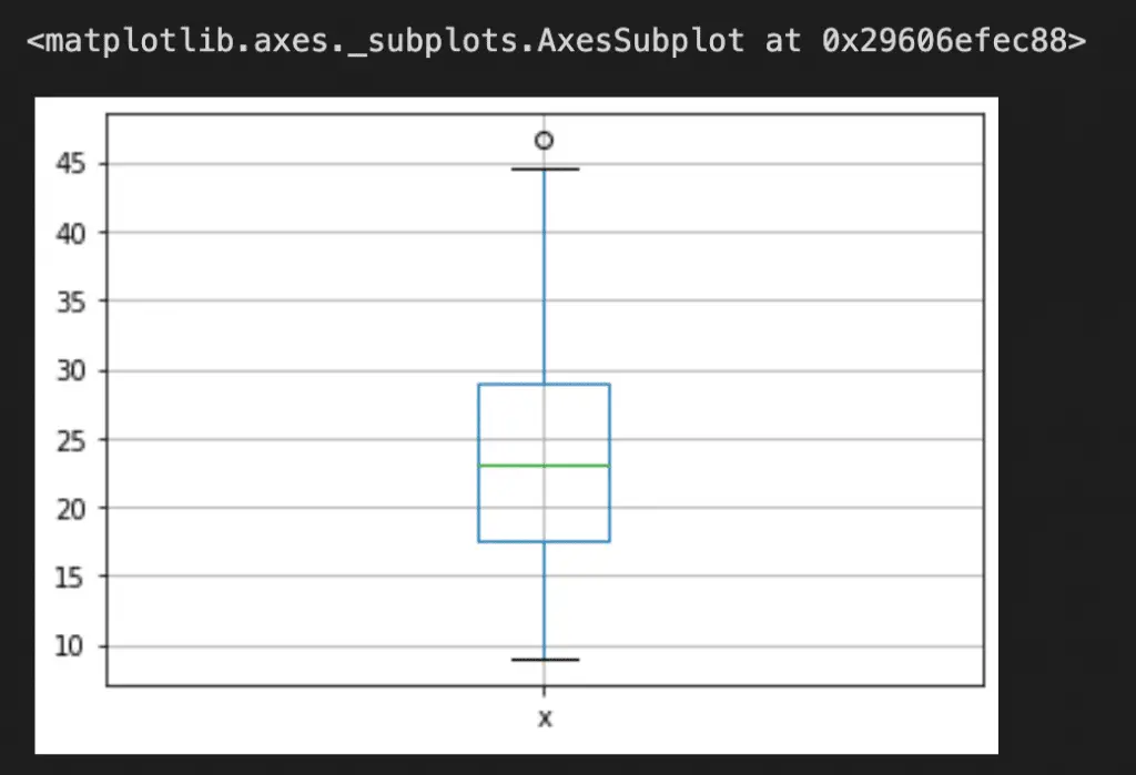
Day 22: plotting.boxplot
I want to introduce a simple method to create a boxplot from the series object called plotting.boxplot.
If you did not know boxplot is, quoting from the Pandas guide boxplot is “a method for graphically depicting groups of numerical data through their quartiles. The box extends from the Q1 to Q3 quartile values of the data, with a line at the median (Q2). The whiskers extend from the edges of the box to show the range of the data. By default, they extend no more than 1.5 * IQR (IQR = Q3 – Q1) from the edges of the box, ending at the farthest data point within that interval. Outliers are plotted as separate dots”.
You only need to pass the series or the data frame, and the numerical columns would be plotted automatically.
import pandas as pd
import seaborn as sns
import matplotlib.pyplot as plt

mpg = sns.load_dataset('mpg')
pd.plotting.boxplot(mpg['mpg'])
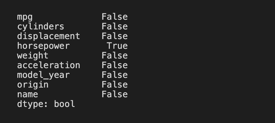
Day 23: any
I would introduce you to a simple yet useful Series and DataFrame method called .any.
What is this method do? So, .any would return a boolean value where it would return True if any of the element is True and returns False if there is no True boolean in the series or column.
It is most useful when we want to check if there are missing values in our dataset. Just look at the example, we chained .isna with .any. Only the horsepower return True because there is a missing data present in this column.
import pandas as pd
import seaborn as sns
import matplotlib.pyplot as plt

mpg = sns.load_dataset('mpg')
mpg.isna().any()
Day 24: where
I want to introduce you to a DataFrame method similar to the one I post previously called .where.
So, this method inversely works compared to the .mask method I post before. Basically it is a method which accepting condition and the one values that did not fill the condition would be replaced.
Just look at the example, I give criteria to look for values below 20 and any values below 20 would keep their values, otherwise, it would be replaced by “More than Twenty”.
import pandas as pd
import seaborn as sns

mpg = sns.load_dataset('mpg')
mpg['mpg'].where(mpg['mpg'] < 20, 'More than Twenty' )
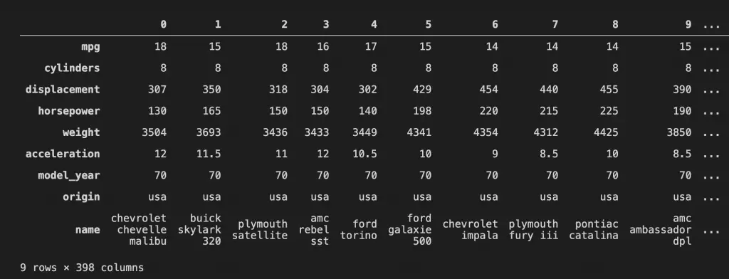
Day 25: Transpose
import pandas as pd
import seaborn as sns

mpg = sns.load_dataset('mpg')
mpg.transpose()
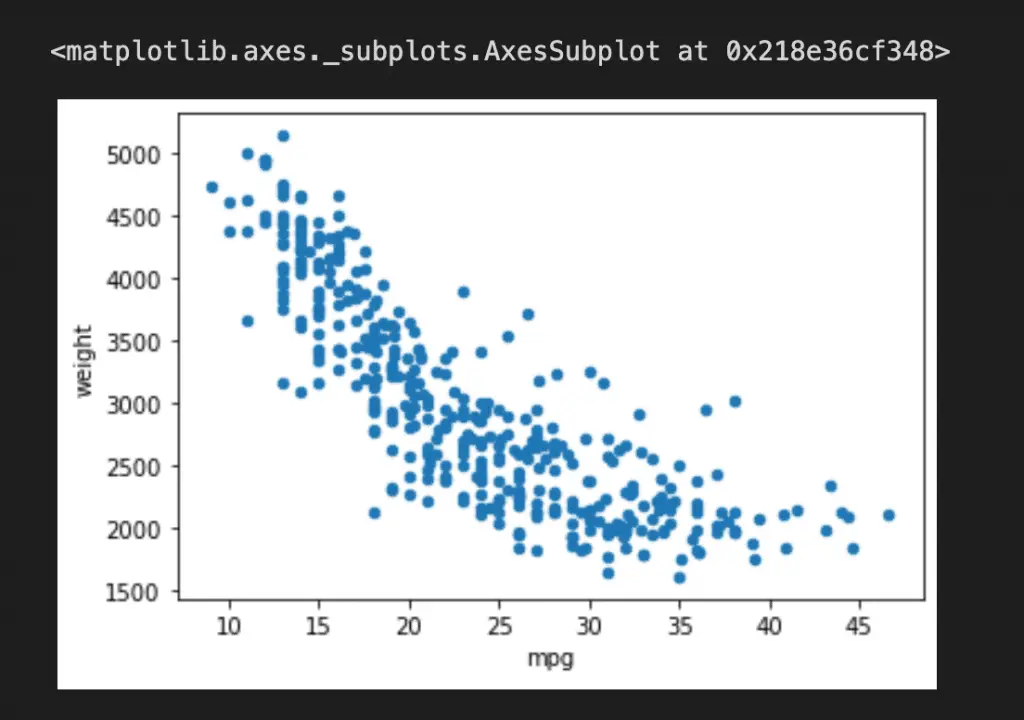
Day 26: plot.scatter
Today I want to introduce a quick plotting method from pandas DataFrame object called plot.scatter.
I am sure many people many know what is scatter plot is, although for you who doesn’t know; it is basically a plot where we plot every data in 2 different numerical columns which the values are visualized in the plot.
We could create a quick scatter plot just by using .plot.scatter in the Data Frame object and pass 2 columns name you want.
import pandas as pd
import seaborn as sns

mpg = sns.load_dataset('mpg')
mpg.plot.scatter('mpg', 'weight')
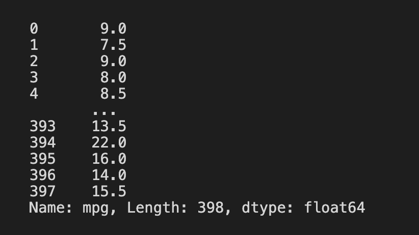
Day 27: transform
Today, I want to introduce a method from the Series and Data Frame object called .transform.
It is a simple function but powerful. The main premise of this function is we pass a function or the aggregation string name and the function is applied on all of the values.
If you used it in the DataFrame object, the function would be applied to every value in every column.
import pandas as pd
import seaborn as sns

mpg = sns.load_dataset('mpg')
mpg['mpg'].transform(lambda x: x/2)
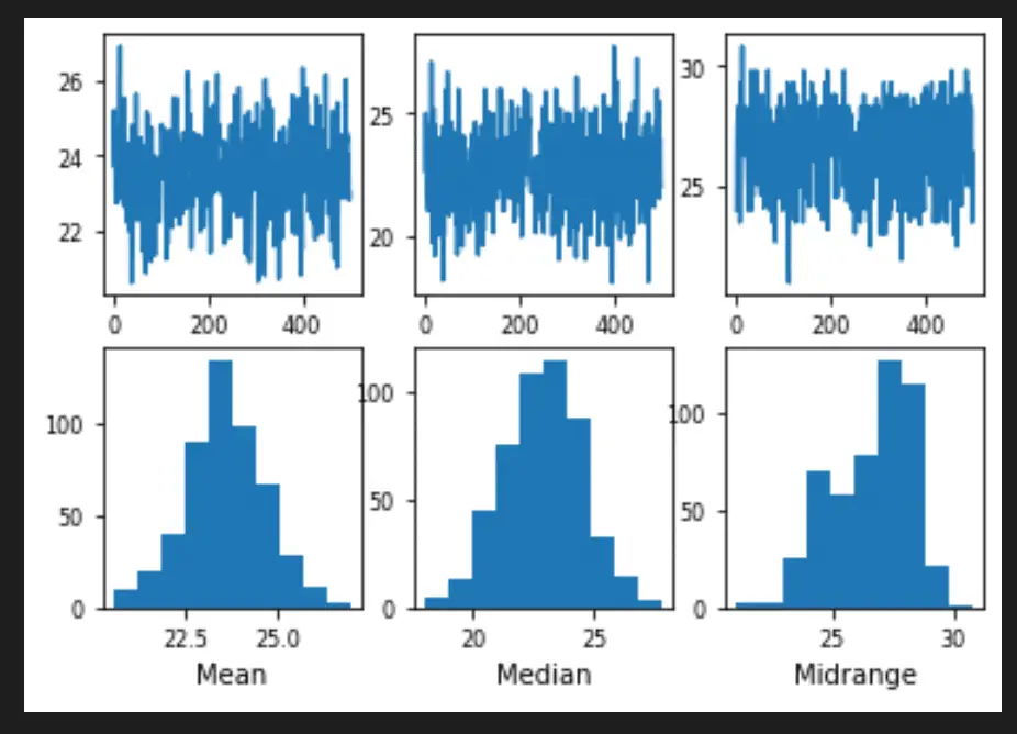
Day 28: bootstrap_plot
Today I want to introduce a unique plotting function from Pandas called .bootstrap_plot.
According to Pandas, the bootstrap plot is used to estimate the uncertainty of a statistic by relying on random sampling with replacement.
In simpler words, it is used to trying to determine the uncertainty in fundamental statistic such as mean and median by resampling the data with replacement (you could sample the same data multiple times).
The boostrap_plot function will generate bootstrapping plots for mean, median and mid-range statistics for the given number of samples of the given size. Just like in the example below.
import pandas as pd
import seaborn as sns

mpg = sns.load_dataset('mpg')
pd.plotting.bootstrap_plot(mpg['mpg'], size = 50, samples = 500)
plt.show()
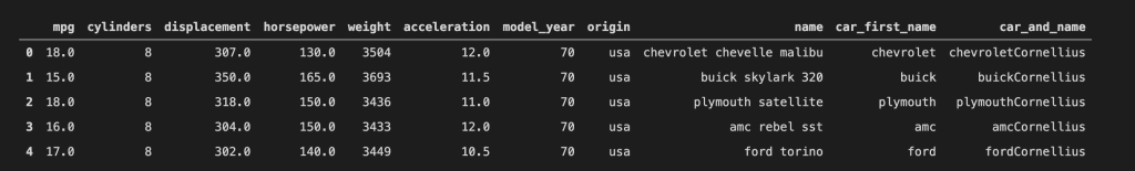
Day 29: pipe
In today pandas post, I want to introduce a method that I encourage people to use more often. The method is .pipe.
So, Pandas encouraged us to use a method chaining to manipulate our data. Normally we would chaining method by passing function in function or method with the method after.
With .pipe function, the chaining method in Pandas DataFrame could decrease the line we write and execute the function faster.
The example of the .pipe method is in the picture below. I create two different functions and chain the method by executing the .pipe twice. This in order to create a chain method and faster execution.
import pandas as pd
import seaborn as sns

mpg = sns.load_dataset('mpg')

#Function to extract the car first name and create a new column called car_first_name
def extract_car_first_name(df):
    df['car_first_name'] = df['name'].str.split(' ').str.get(0)
    return df

#Function to add my_name after the car_first_name and create a new column called car_and_name
def add_car_my_name(df, my_name = None):
    df['car_and_name'] = df['car_first_name'] + my_name

mpg.pipe(extract_car_first_name).pipe(add_car_my_name, my_name = 'Cornellius')

mpg.head()
Day 30: show_versions
On the last day, I want to show you a special function from pandas called .show_versions. Well, what is this function do?
The function giving us info about the hosting operation system, pandas version, and versions of other installed relative packages. It provides useful information especially when you messing around with related packages and also important for bug reports.
import pandas as pd

pd.show_versions(True)

So. today is was last day of my 30 days of pandas post. It was a quite a fun and insightful activity for me. I enjoyed creating content like this for people and I hope it was useful for anybody that I have reached.

Cornellius Yudha Wijaya is a Data Scientist in Allianz Life Indonesia and often writing about Data Science in his free time. He holds a Biology M.Sc. Degree from Uppsala University and have since managed to teach people how to break into the Data Science industry.