
In this tutorial, you will learn about the PCA machine learning algorithm using Python and Scikit-learn.
What is Principal Component Analysis (PCA)?
PCA, or Principal component analysis, is the main linear algorithm for dimension reduction often used in unsupervised learning. In simple words, PCA tries to reduce the number of dimension whilst retaining as much variation in the data as possible.
This algorithm identifies and discards features that are less useful to make a valid approximation on a dataset.
Introduction to PCA in Python
Principal Component Analysis (PCA) is a technique used in Python and machine learning to reduce the dimensionality of high-dimensional data while preserving the most important information.
Simply put, PCA makes complex data simpler by taking a lot of information and finding the most important parts. This helps to fight the curse of dimensionality.
Install Scikit-Learn to use PCA in Python
For this tutorial, you will also need to install Python and install Scikit-learn library from your command prompt or Terminal.
$ pip install scikit-learnSimplest Example of PCA in Python
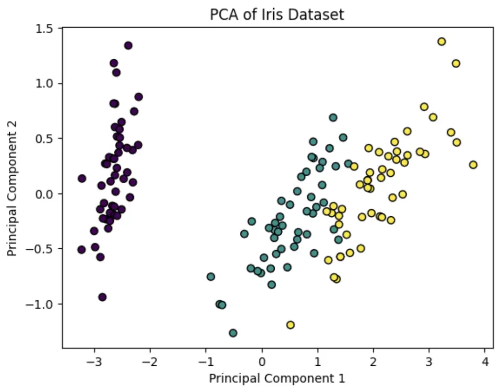
Here is a simple example of how to use Python PCA algorithm in Scikit-learn to reduce the features of the Iris dataset and plot a 2D graph.
import matplotlib.pyplot as plt
from sklearn.decomposition import PCA
from sklearn.datasets import load_iris

# Load Iris dataset
iris = load_iris()
X = iris.data
y = iris.target

# Apply PCA with two components (for 2D visualization)
pca = PCA(n_components=2)
X_pca = pca.fit_transform(X)

# Plot the results
plt.scatter(X_pca[:, 0], X_pca[:, 1], c=y, cmap='viridis', edgecolor='k')
plt.title('PCA of Iris Dataset')
plt.xlabel('Principal Component 1')
plt.ylabel('Principal Component 2')
plt.show()
Getting Started with Principal Component Analysis in Python
In this Python tutorial, we will perform principal component analysis on the Iris dataset using Scikit-learn. We will now install Scikit-learn and load the built-in Iris dataset.
- Explore the Iris Dataset
- Load the Dataset with Sciki-learn
- Perform Data Preprocessing in Python
- Perform Dimension Reduction using PCA in Python
- Give Names for Your Plot by Mapping targets to Principal Components
- Plot the 2D PCA Graph
1. Explore the Python Dataset (Iris)
The Iris dataset is useful to visualize how Principal Component Analysis works.
The iris dataset contains 4 features (predictor variables) describing 3 species of flowers (targets).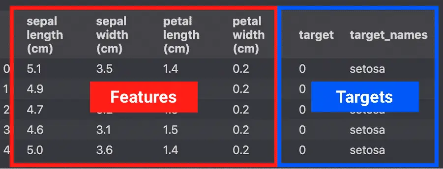
2. Load the Iris Dataset with Scikit-Learn
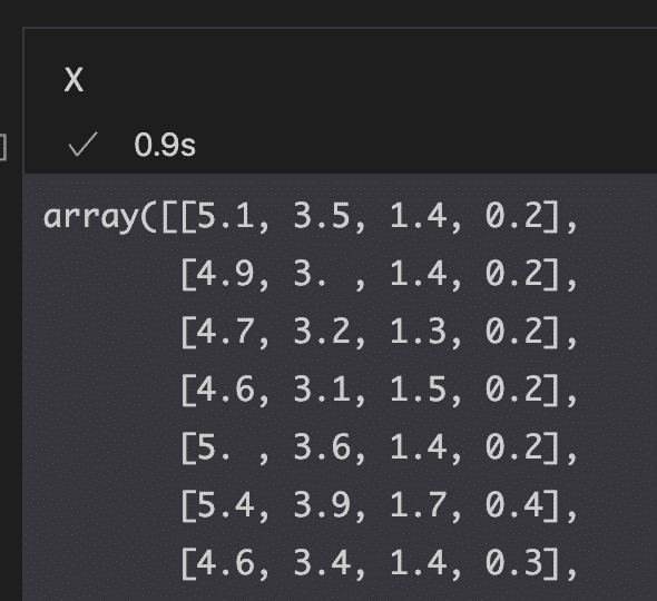
To load the Iris dataset from Scikit-learn, let’s load features and targets as arrays stored in their respective X and y variables.
from sklearn import datasets

# load features and targets separately
iris = datasets.load_iris()
X = iris.data
y = iris.target
3. Perform Data Preprocessing in Python
Before running PCA, let’s perform very basic data preprocessing and scale the data using StandardScaler.
# data scaling
from sklearn.preprocessing import StandardScaler
x_scaled = StandardScaler().fit_transform(X)
StandardScaler will standardize the features by removing the mean and scaling to unit variance so that each feature has μ = 0 and σ = 1.
Converting this: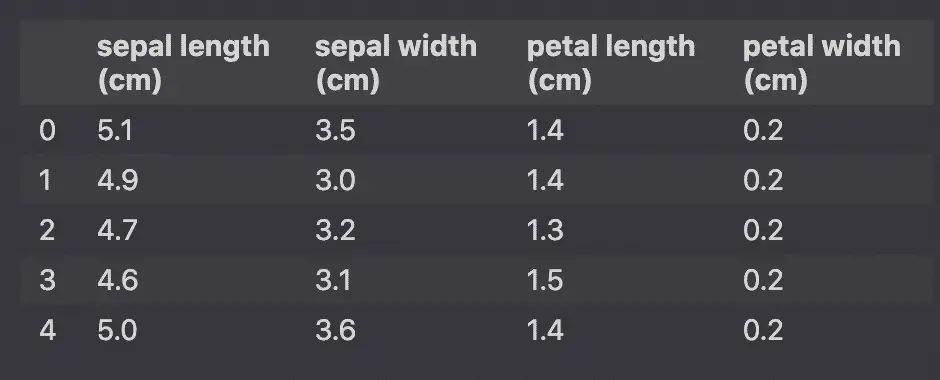
Into this: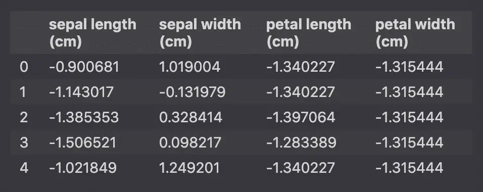
4. Perform Dimension Reduction using PCA in Python
To perform dimension reduction in Python, import PCA from sklearn.decomposition and use the fit_transform() method on the PCA() object. The n_components argument tells the number of dimensions to keep.
We have seen that the Iris dataset contains 4 features, making it a 4-dimensional dataset. Not all features are necessarily useful for the prediction. Therefore, we can remove those noisy features and make a faster model.
The n_components argument will define the number of components that we want to reduce the features to.
# Dimention Reduction
pca = PCA(n_components=2)
pca_features = pca.fit_transform(x_scaled)

# Show PCA characteristics
print('Shape before PCA: ', x_scaled.shape)
print('Shape after PCA: ', pca_features.shape)
Shape before PCA: (150, 4)
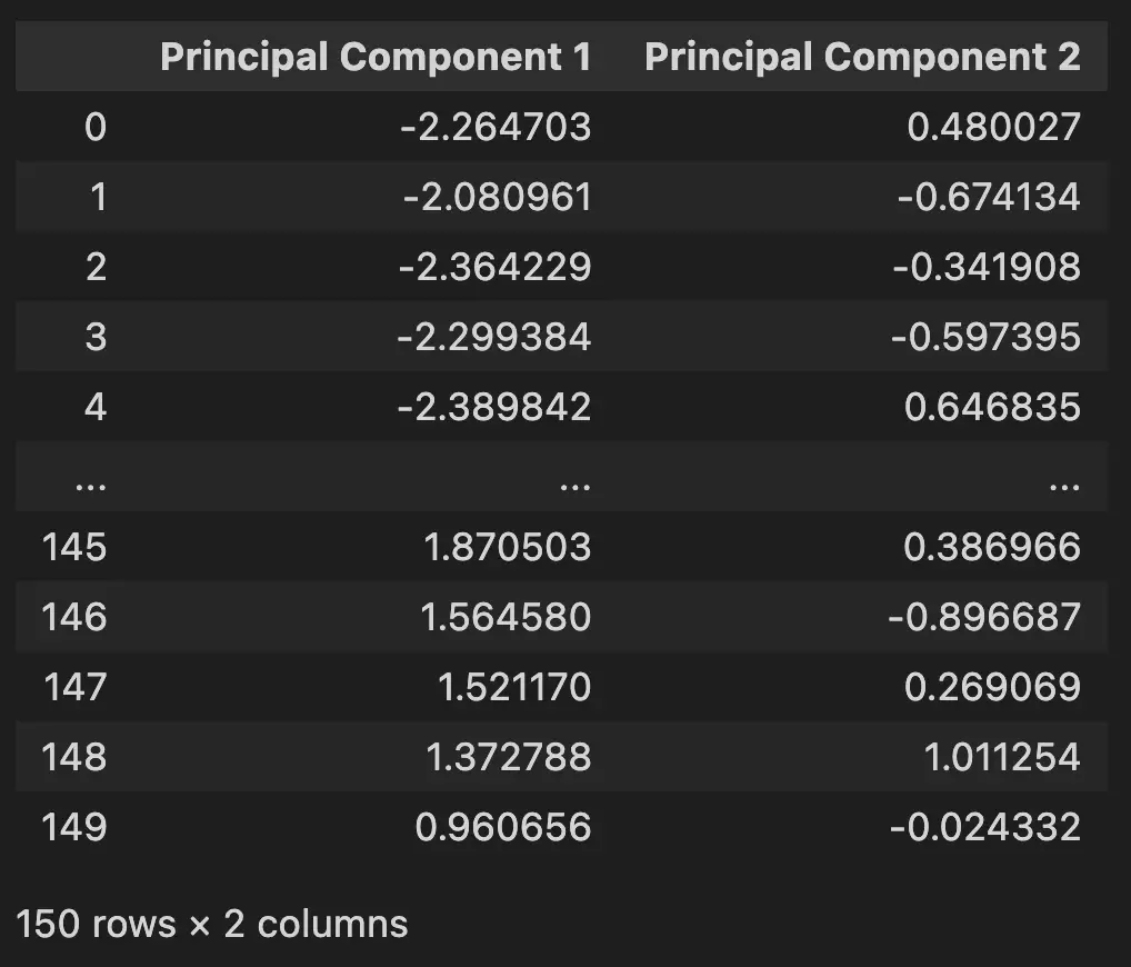
Shape after PCA: (150, 2)For better understanding, PCA converted this data with 4 features.
Into this data with 2 principal components.
# Create PCA DataFrame
pca_df = pd.DataFrame(
    data=pca_features,
    columns=[
        'Principal Component 1',
        'Principal Component 2'
        ])
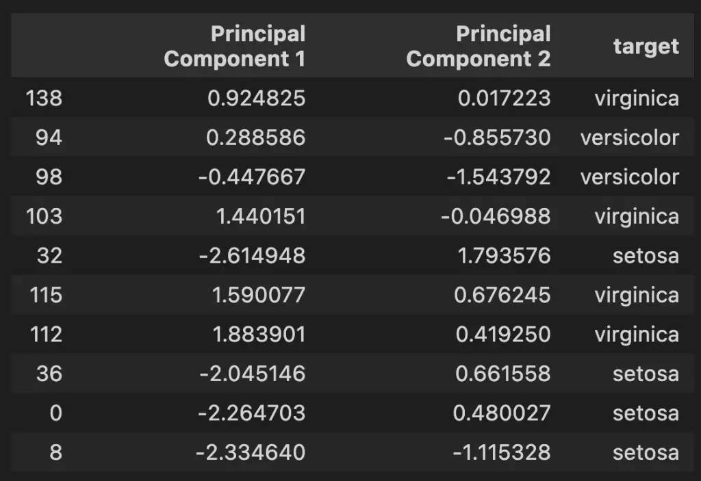
5. Give Names for Your Plot by Mapping targets to Principal Components
We will prepare the PCA Dataframe for visualization by mapping the target names to the PCA features.
# Map target names to targets
target_names = {
    0:'setosa',
    1:'versicolor',
    2:'virginica'
}

pca_df['target'] = y
pca_df['target'] = pca_df['target'].map(target_names)
pca_df.sample(10)
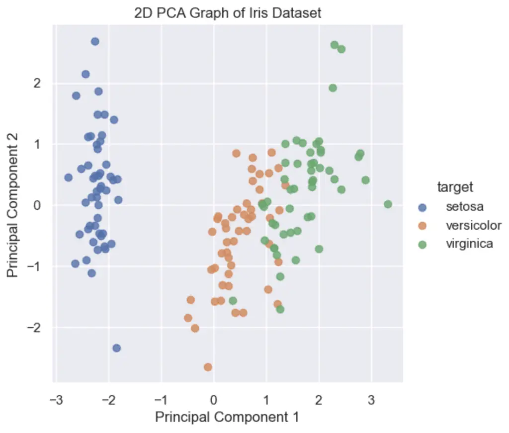
6. Plot the 2D PCA Graph
To plot the 2D PCA graph, use the Principal Component DataFrame to Seaborn’s lmplot() function.
import matplotlib.pyplot as plt
import seaborn as sns
sns.set()
# Plot 2D PCA Graph
sns.lmplot(
    x='Principal Component 1',
    y='Principal Component 2',
    data=pca_df,
    hue='target',
    fit_reg=False,
    legend=True
    )

plt.title('2D PCA Graph of Iris Dataset')
plt.show()
Follow this tutorial if you want to plot a 3D PCA Graph instead.
What is Next?
- Identify Important PCA Features
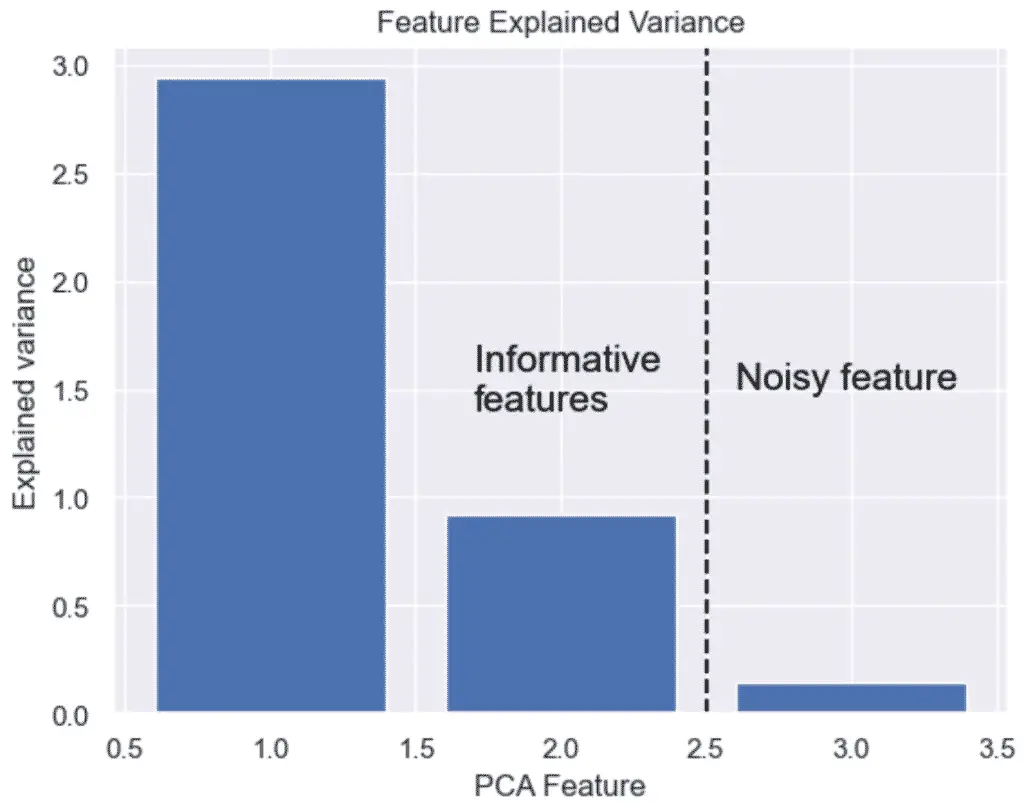
- Plot the Feature Explained Variance
- Plot a Scree Plot
- Make PCA Biplots
- PCA Project: Clustering and De-duplication of web pages using KMeans and TF-IDF
Additional PCA Learning Materials
- Understand How the PCA Algorithm Works in Python
- Understand What the Explained Variance Is
- Understand the Different Types of PCA Plots
- Learn About the Common Methods used in PCA
- PCA using Python (scikit-learn) by Michael Galarnyk on Towardsdatascience
- Principal Component Analysis Visualization by Prasad Ostwal
- Performing and visualizing the Principal component analysis (PCA) from PCA function and scratch in Python by Renesh Bedre
How Many Dimensions Should You Reduce Your Data with PCA?
To decide the number of dimensions that you should reduce your data to, you should make a cumulative explained variance plot (scree plot) to show each of your individual component variance on top of your cumulative variance.
We could decide to keep 90%+ of the variance and thus keep 3 Principal components.

Full PCA Code
import pandas as pd
from sklearn import datasets
from sklearn.preprocessing import StandardScaler
from sklearn.decomposition import PCA
import matplotlib.pyplot as plt
import seaborn as sns
sns.set()

# load features and targets separately
iris = datasets.load_iris()
X = iris.data
y = iris.target

# Data Scaling
x_scaled = StandardScaler().fit_transform(X)

# Dimention Reduction
pca = PCA(n_components=2)
pca_features = pca.fit_transform(x_scaled)

# Show PCA characteristics
print('Shape before PCA: ', x_scaled.shape)
print('Shape after PCA: ', pca_features.shape)
print('PCA Explained variance:', pca.explained_variance_)

# Create PCA DataFrame
pca_df = pd.DataFrame(
    data=pca_features,
    columns=[
        'Principal Component 1',
        'Principal Component 2'
        ])


# Map target names to targets
target_names = {
    0:'setosa',
    1:'versicolor',
    2:'virginica'
}

pca_df['target'] = y
pca_df['target'] = pca_df['target'].map(target_names)
pca_df.sample(10)

# Plot 2D PCA Graph
sns.lmplot(
    x='Principal Component 1',
    y='Principal Component 2',
    data=pca_df,
    hue='target',
    fit_reg=False,
    legend=True
    )

plt.title('2D PCA Graph of Iris Dataset')
plt.show()


# Bar plot of explained_variance
plt.bar(
    range(1,len(pca.explained_variance_)+1),
    pca.explained_variance_
    )

plt.xlabel('PCA Feature')
plt.ylabel('Explained variance')
plt.title('Feature Explained Variance')
plt.show()
Python PCA and Machine Learning Definitions
| Principal Component Analysis | Linear algorithm for dimension reduction |
| PCA Python library | sklearn.decomposition.PCA |
| Plot PCA in Python | Searborn lmplot() can be used |
| PCA usage | Speed and simplicity |
Video Series on PCA
Conclusion
Congratulations, you now have learned one of the most important dimension reduction techniques.
With principal component analysis (PCA) you have optimized machine learning models and created more insightful visualizations.
You also learned how to understand the relationship between each feature and the principal component by creating 2D and 3D loading plots and biplots.

SEO Strategist at Tripadvisor, ex- Seek (Melbourne, Australia). Specialized in technical SEO. Writer in Python, Information Retrieval, SEO and machine learning. Guest author at SearchEngineJournal, SearchEngineLand and OnCrawl.